Paper Summary: Very Deep Convolutional Networks for Large-Scale Image Recognition

Abstract For Summary

The paper named “Very Deep Convolutional Networks for Large-Scale Image Recognition”, also known as “VGGNet”, proposes six different Convolutional Neural Network models (named A, A-LRN, B, C, D, E) and compares them based on architectural differences and results on top-1 and top-5 error rates. Also the authors introduces different, from other ImageNet models, data augmentation method based on varying image scales or widely known as “image jittering”. Furthermore, the model uses different evaluation techniques, dense versus multi-crop versus multi-crop & dense. At the end, I will show a simple VGGNet model code written in PyTorch.

ImageNet 2014

VGGNet is not the winner of classification task in 2014’s ILSVRC (ImageNet Large Scale Visual Recognition Competition). To see who were the winners (for more information):

• Task 1a: Object detection with provided training data: NUS
• Task 1b: Object detection with additional training data: GoogLeNet
• Task 2a: Classification+localization with provided training data: VGGNet
• Task 2b: Classification+localization with additional training data: Adobe-UIUC

The ImageNet 2014 dataset includes images of 1000 classes and split into three sets: training set has 1.3M images, validation set has 50K images, test set 100K images with held-out class labels. Classification performance is evaluated on two measures: top-1 error and top-5 error. In top-1 error, you check if the top class probability is the same as the target label; in top-5 error, you check if the target label is one of your top 5 predictions.

Model Architecture and Configurations

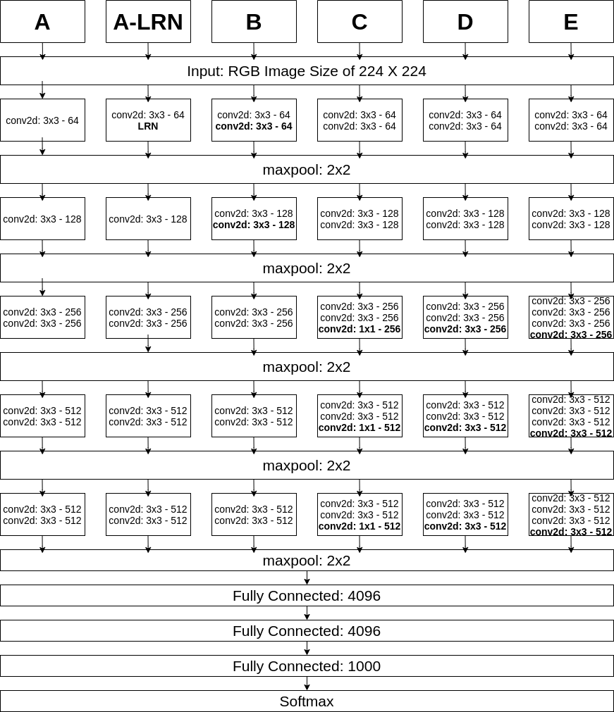
As we can see above, model has 6 configurations;

• A is 11 layered.
• A-LRN is 11 layered but have Local Response Normalization.
• B is 13 layered.
• C is 16 layered but have 1x1 convolutional layers.
• D is 16 layered but 1x1 convolutional layers in C are replaced with 3x3 convolutional layers.
• E is 19 layered.

For being more clear about figures, nonlinear ReLU layers was not shown in above figure.

During training, the input is RGB images of fixed-size 224x224. The only preprocessing for data is subtracting the mean EGB value from each pixel. Max-poolings are performed over a 2x2 kernel with stride of 2. All hidden non-linear activation functions are ReLU. Fully connected layers are designed as 4096 \(\rightarrow\) 4096 \(\rightarrow\) 1000 (1000 class), and softmax is used in output layer. Except for configuration C all kernels have size of 3x3 with stride of 1 in convolutional layers. C layer also has 1x1 convolutional layers. Also the padding is 1 pixel for 3x3 convolutional layers. The configuration A-LRN is the same with configuration A except for Local Response Normalization (LRN) layer. But LRN does not improve the performance on ILSVRC dataset, but leads into increased memory consumption and computation time.

Going Smaller With Kernel Sizes

Rather than using relatively large kernel sizes in first convolutional layers (e.g. 5x5: stride 2, 7x7: stride 2, 11x11: stride 4), VGGNet uses three 3x3 convolutional laters which is equivalent with one 7x7 convolutional layer. Also using 3 3x3 convolutional layers rather than one 7x7 convolutional layer has benefits:

• Adding more non-linearity: more non-linear rectified unit (ReLU).
• Decreasing number of parameters: with \(C\) channnel, \(49C^2\) reduced to \(27C^2\).
• Using 1x1 convolutional layers is a way to increase the non-linearity without affecting the receptive fileds of the convolutional layers.

Training

Training configurations is like this:

• Objective function is multinomial logistic regression.
• Optimizer is mini-batch gradient descent with momentum.
  • Batch size of 256.
  • Momentum of 0.9.
• The L2 regularizer is used.
  • \(\lambda\) = \(5\times 10^{-4}\)
• Dropout is used.
  • p = 0.5.
• Learning rate \(\eta = 10^{-2}\)
  • Learning rate is increased by factor 10 when performance on validation set not improved (in paper, 3 times).
• 74 epochs.

Varying Image Scales

If we only train the network at the same scale, we might miss the detection or have the wrong classification for the objects with other scales. For this problem multi-scale evaluation is propoesed.

• Single-Scale Training / Multi-Scale Training with Single-Scale Evaluation
  • For training image size \(S\) and \(Q\), test image size is set as \(Q = S\) for fixed \(S\), and \(Q=0.5(S_{min}+S_{max})\) for \(S \in [S_{min},S_{max}]\)
  • Since the model accepts fixed sized images; this means that during training, the image is rescaled to set the length of the shortest side to \(S\) and then cropped; in other words, image is scaled into range from 256x256 to 512x512 then cropped to 224x224.
  • You can clearly see that scale jittering in training gives us better results in ILSVRC Dataset.
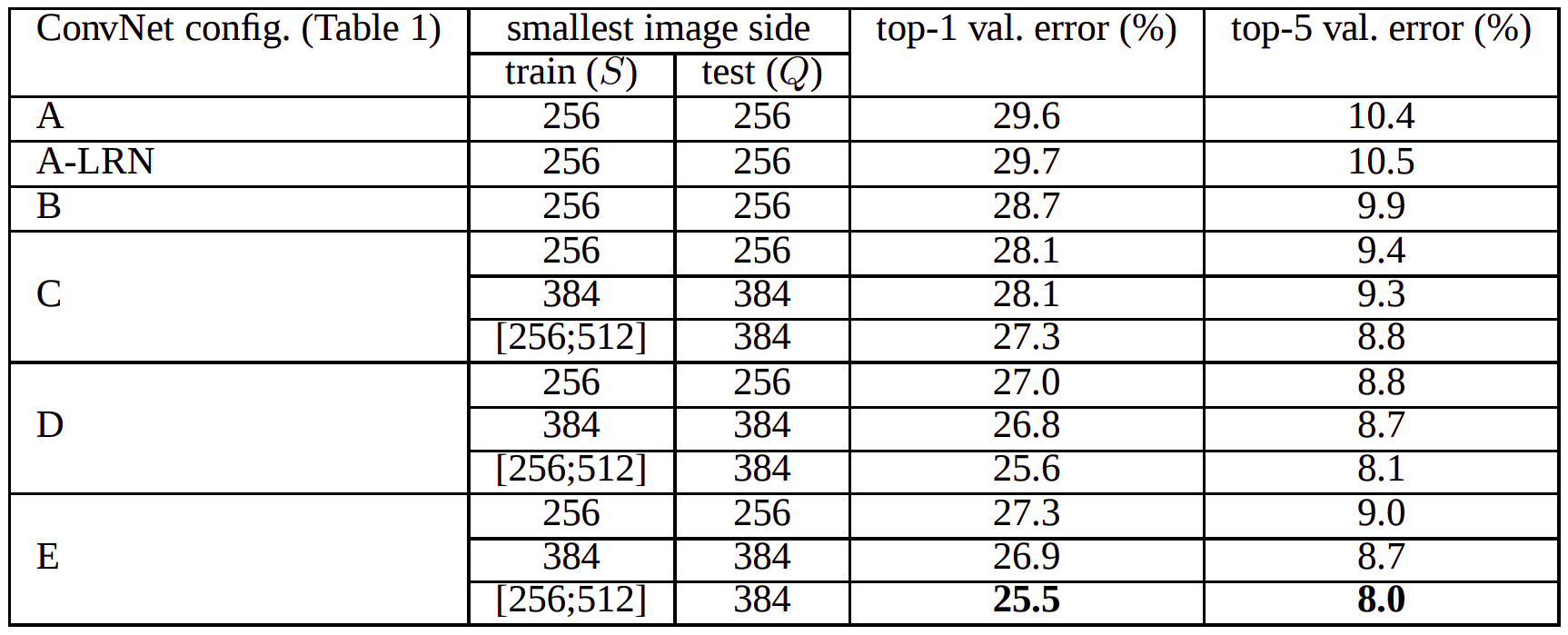
• Single-Scale Training / Multi-Scale Training with Multi-Scale Evaluation
  • Model is evaluated with for fixed \(S\;\), \(Q = \{S-32, S, S+32\}\); for \(S \in [S_{min},S_{max}]\), \(Q=\{S_{min}, 0.5(S_{min}+S_{max}), S_{max}\}\)
  • You can clearly see that scale jittering in testing gives us better results in ILSVRC Dataset.
• Dense versus Multi-Crop Evaluation
  • In dense evaluation, the fully connected layers are converted to convolutional layers at test time, and the uncropped image is passed through the fully convolutional net to get dense class scores. Scores are averaged for the uncropped image and its flip to obtain the final fixed-width class posteriors.
  • This is compared against taking multiple crops of the test image and averaging scores obtained by passing each of these through the CNN.
  • Multi-crop evaluation works slightly better than dense evaluation, but the methods are somewhat complementary as averaging scores from both did better than each of them individually.
  • The authors hypothesize that this is probably because of the different boundary conditions: when applying a ConvNet to a crop, the convolved feature maps are padded with zeros, while in the case of dense evaluation the padding for the same crop naturally comes from the neighbouring parts of an image (due to both the convolutions and spatial pooling), which substantially increases the overall network receptive field, so more context is captured.
  • We can see this performance results clearly.

Combining ConvNet Models and Final Reports

The above models are evaluated individually. With ConvNet Fusion, authors combine the outputs of several models by averaging their soft-max class posteriors. This improves model performance. Visual Geometry Group reached 23.7 top-1 val error after ILSVRC submission! You can see the table from paper to see what ensembles and performances:

My Thoughts

• Model was constructed very thoughtful, design of image scales, and dense v/s multi-crop evaluations is very important.
• Also it is tricky that authors began with training the configuration A, shallow enough to be trained with random initialisation; Then, when training deeper architectures, they initialised the first four convolutional layers and the last three fully connected layers with the layers of net A and the intermediate layers were initialised randomly.
• Using small kernels and reducing slowly spatial resolution of the feature maps are important for extracting features from images.
• Authors showed that using Local Response Normalization does not improve the performance on the ILSVRC dataset.
• Increasing the nonlinearity of the decision function without affecting the receptive fields of the conv. layers is showed with 1x1 Convolutional layers.
• Also; paper is readable, the desing and wording of paper is so clean.

A more deeper convolutional architecture shows its power.

A Minimalist Implementation On CIFAR100

Now we will make a minimalist implementation on CIFAR100 to get about 70% accuracy (PyTorch 1.7.0+cu101). Start with imports:

import torch
import torchvision as tv
import numpy as np
import torch.nn as nn
import torchvision.transforms as transforms
import torch.optim as optim
import matplotlib.pyplot as plt

Then compute the mean and standard deviation of RGB channels to normalize the data for better performance. Befor doing this, define our dataset as a dataloader object in PyTorch.

device = torch.device("cuda" if torch.cuda.is_available() else "cpu")
transform_stats = transforms.Compose([
    transforms.ToTensor(),
])
trainset_stats = tv.datasets.CIFAR100(root='./data/CIFAR100', train=True, download=True, transform=transform_stats)
trainloader_stats = torch.utils.data.DataLoader(trainset_stats, 200, num_workers=2)

Now compute the mean

dim_sum = 0
h = 0
w = 0
for i, (input, target) in enumerate(trainloader_stats):
    input, target = input.to(device), target.to(device)
    if i == 0:
        h, w = input.size(2), input.size(3)
        dim_sum = input.sum(dim=(0, 2, 3), keepdim=True)
    else:
        dim_sum += input.sum(dim=(0, 2, 3), keepdim=True)
mean = dim_sum/len(trainset_stats)/h/w
print('mean: %s' % mean.view(-1))

and the standard deviation

dim_sum = 0
for i, (input, target) in enumerate(trainloader_stats):
    input,target = input.to(device), target.to(device)
    if i == 0:
        dim_sum = (input - mean).pow(2).sum(dim=(0, 2, 3), keepdim=True)
    else:
        dim_sum += (input - mean).pow(2).sum(dim=(0, 2, 3), keepdim=True)
std = torch.sqrt(dim_sum/(len(trainset_stats) * h * w - 1))
print('std: %s' % std.view(-1))

the mean should be [0.5071, 0.4865, 0.4409] and the standard devition should be [0.2673, 0.2564, 0.2762].

Now prepare our trainloader and testloader for training the model. RandomCrop and RandomHorizontalFlip are used for data augmentation.

batch_size = 200
transform_train = transforms.Compose([
        transforms.RandomCrop(32, padding=4),
        transforms.RandomHorizontalFlip(),
        transforms.ToTensor(),
        transforms.Normalize((0.5071, 0.4865, 0.4409), (0.2673, 0.2564, 0.2762)),
    ])

transform_test = transforms.Compose([
        transforms.ToTensor(),
        transforms.Normalize((0.5071, 0.4865, 0.4409), (0.2673, 0.2564, 0.2762)),
    ])

trainset = tv.datasets.CIFAR100(root='./data/CIFAR100', train=True,
                                        download=True, transform=transform_train)

trainloader = torch.utils.data.DataLoader(trainset, batch_size=batch_size,
                                          shuffle=True, num_workers=2)

testset = tv.datasets.CIFAR100(root='./data/CIFAR100', train=False,
                                       download=True, transform=transform_test)

testloader = torch.utils.data.DataLoader(testset, batch_size=batch_size,
                                         shuffle=False, num_workers=2)

Now it is time to implement our minimalist VGGNet and its configurations.

class MyOwnNets(nn.Module):
  def __init__(self,features,init_h):
    super(MyOwnNets,self).__init__()
    self.features = features
    self.classifier = nn.Sequential(
        nn.Dropout(p=0.5,inplace=False),
        nn.Linear(in_features = 512,out_features = 512),
        nn.ReLU(inplace=True),
        nn.Dropout(p=0.5,inplace=False),
        nn.Linear(in_features = 512,out_features = 512),
        nn.ReLU(inplace=True),
        nn.Linear(512,init_h),
        )
    for module in self.modules():
      if isinstance(module, nn.Conv2d):
        n = module.kernel_size[0] * module.kernel_size[1] * module.out_channels
        module.weight.data.normal_(0,math.sqrt(2. / n))
        module.bias.data.zero_()

  def forward(self,x):
    out = self.features(x)
    out = out.view(out.size(0),-1)
    out = self.classifier(out)
    return out

  @staticmethod
  def addLayer(config,batch_norm=False,in_channels=3):
    if type(config) != list:
      raise TypeError("Configuration must be in type of list. {}".format(type(config)))
    else:
      layers = []
      for v in config:
        if v == 'MP':
          layers += [nn.MaxPool2d(kernel_size=2,stride=2)]
        else:
          if type(v) is not int:
            raise TypeError("Except MaxPool, configuration feature type must be integer.")
          else:
            conv2d = nn.Conv2d(in_channels=in_channels, 
                                out_channels=v, kernel_size=3,
                                padding = 1)
            if batch_norm:
              layers += [conv2d, nn.BatchNorm2d(v), nn.ReLU(inplace=True)]
            else:
              layers += [conv2d, nn.ReLU(inplace=True)]
            in_channels = v
      return nn.Sequential(*layers)

  @staticmethod
  def __config__():
    return  {'11': [64, 'MP', 128, 'MP', 256, 256, 'MP', 512, 512, 'MP', 512, 512, 'MP'],
             '13': [64, 64, 'MP', 128, 128, 'MP', 256, 256, 'MP', 512, 512, 'MP', 512, 512, 'MP'],
             '16': [64, 64, 'MP', 128, 128, 'MP', 256, 256, 256, 'MP', 512, 512, 512, 'MP', 512, 512, 512, 'MP'],
             '19': [64, 64, 'MP', 128, 128, 'MP', 256, 256, 256, 256, 'MP', 512, 512, 512, 512, 'MP', 512, 512, 512, 512, 'MP'],
             }

Let’s initialize our model objects

config = MyOwnNets.__config__()
model11 = MyOwnNets(MyOwnNets.addLayer(config = config['11'],batch_norm = True, in_channels = 3),100).to(device)
model13 = MyOwnNets(MyOwnNets.addLayer(config = config['13'],batch_norm = True, in_channels = 3),100).to(device)
model16 = MyOwnNets(MyOwnNets.addLayer(config = config['16'],batch_norm = True, in_channels = 3),100).to(device)
model19 = MyOwnNets(MyOwnNets.addLayer(config = config['19'],batch_norm = True, in_channels = 3),100).to(device)

Defining objective function as Cross Entropy Loss, we use optimizer as AdaM. Learning rate scheduler with weight decay of 1e-5 is used for better performance.

CUDA = torch.cuda.is_available()
criterion = nn.CrossEntropyLoss()
optimizer = optim.Adam(model13.parameters(),lr=0.01, weight_decay=1e-5)
scheduler = optim.lr_scheduler.OneCycleLR(optimizer, 0.01, epochs=epochs, steps_per_epoch=len(trainloader))

The model 13 gets highest accuracy on CIFAR100, writing the training and evaluating loop:

epochs = 120
training_loss = []
training_accuracy= []
test_loss = []
test_accuracy = []

for epoch in range(epochs):
  correct = 0
  iterations = 0
  each_loss = 0.0

  model13.train()
  for i,(inputs, targets) in enumerate(trainloader): 
    if CUDA:
      inputs = inputs.cuda()
      targets = targets.cuda()
    outputs = model13.forward(inputs)
    loss = criterion(outputs, targets)
    each_loss+=loss.item()

    optimizer.zero_grad()
    loss.backward()
    optimizer.step()
    scheduler.step()
    _, predicted=torch.max(outputs,1)
    correct += (predicted == targets).sum().item()
    iterations += 1
  training_loss.append(each_loss/iterations)
  training_accuracy.append(100 * correct/len(trainset))

    
  each_loss_test = 0.0
  iterations = 0 
  correct = 0
  model13.eval()
  for i,(inputs, targets) in enumerate(testloader):
      if CUDA: 
          inputs = inputs.cuda()
          targets = targets.cuda()
      outputs= model13.forward(inputs)
      loss = criterion(outputs, targets)
      each_loss_test+=loss.item()

      _, predicted=torch.max(outputs,1)
      correct += (predicted == targets).sum().item()
      iterations += 1

  test_loss.append(each_loss_test/iterations)
  test_accuracy.append(100 * correct/len(testset))
  print("Epoch {}/{} - Training Loss: {:.3f} - Training Accuracy: {:.3f} - Test Loss: {:.3f} - Test Accuracy: {:.3f}"
  .format(epoch+1,epochs,training_loss[-1],training_accuracy[-1],test_loss[-1],test_accuracy[-1]))

The final loss and accuracy on test and train set: Epoch 120/120 - Training Loss: 0.251 - Training Accuracy: 92.712 - Test Loss: 1.494 - Test Accuracy: 70.720

References

• Very Deep Convolutional Networks for Large-Scale Image Recognition
• Going Deeper With Convolutions
• Review: VGGNet — 1st Runner-Up (Image Classification), Winner (Localization) in ILSVRC 2014
• Multiple Crops At Test Time
• ImageNet Large Scale Visual Recognition Challenge 2014 (ILSVRC2014)
• Deep Learning Top Research Papers List