
![]()
x-tagger is a Natural Language Processing library for token classification (POS Tagging etc.). The reason why I called “in its simplest form” is the highest abstraction of it. You can train models and make inference in 5-10 lines of code. Other powerful feature of x-tagger is that it support most common dataset types. What does it mean? For example, torchtext is a common library for PyTorch for Natural Language Processing. Or, it is easy to train huggingface transformers models with huggingface datasets.
x-tagger packs all of these powerful features together. To train a x-tagger model, you need a most simplest form of a POS tagging dataset. In this post, I call it as “x-tagger dataset” but it is nothing but list of tuple lists:
[
[('It', 'PRON'), ('was', 'VERB'), ('outrageous', 'ADJ'), ('.', '.')],

[('``', '.'), ('Both', 'DET'), ('sides', 'NOUN'), ('are', 'VERB'),
 ('taking', 'VERB'), ('action', 'NOUN'), ('.', '.'), ("''", '.')],
...
]
x-tagger is currently in beta release. It supports only Hidden Markov Model, Long Short-Term Memory and BERT.
Tagging With Hidden Markov Model
Hidden Markov Model (HMM) is a statistical Markov model with Markov assumption:
\[P(q_i = \beta \mid q_1 q_2 ...q_{i-1}) \approx p(q_i = \beta \mid q_{i-1})\]Hidden Markov Model for tagging allows us to talk about both observed words (events) and part-of-speech tags (hidden events) that we think of as causal factors in our probabilistic model. Formally defined:
\[\begin{align} Q &= q_1 q_2 q_3 ... q_n \;\;\; &\text{states}\\ A &= a_{11}...a_{ij}...a_{nn} \;\;\; &\text{transition probability matrix}\\ O &= o_1 o_2...o_T \;\;\; &\text{a sequence of T observations}\\ B &= b_i(o_t) \;\;\; &\text{emission probabilities}\\ \pi &= \pi_1,..., \pi_n \;\;\; &\text{initial distribution over states}\\ \end{align}\]For token classification, transition probability means “probability of tag \(t_i\) with observing \(t_{i-1}\)”:
and emission probability means “probability of word \(w_i\) with observing its tag \(t_i\)”:
\[p(w_{i} \mid t_{i}) = \frac{\text{count}(t_{i}, w_{i})}{\text{count}(t_{i})}\]The “training procedure” of HMM is calculating emission and transition probabilities. This probabilities is obtained from tagged training dataset. The formulations of these probabilites is based on bigram Markov assumption. x-tagger has bigram and trigram options.
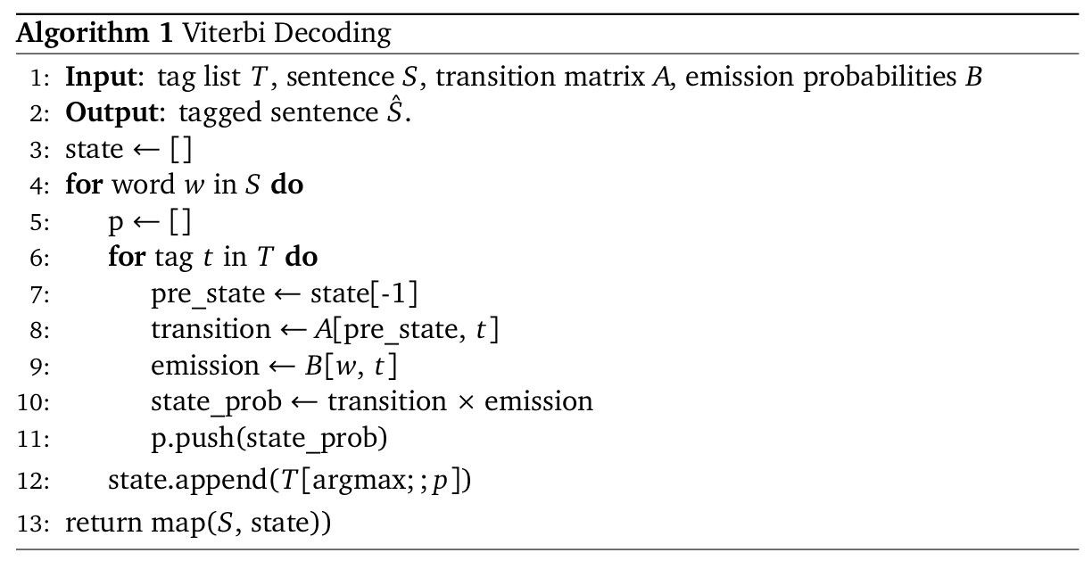
Tagging unobserved samples or evaluation is done by Viterbi Decoding with dynamical programming in x-tagger.
The decoding is to choose the tag sequence \(\mathbf{t}\) that is most probable given the observation sequence of \(n\) words \(\mathbf{w}\):
\[\hat{\mathbf{t}} = \underset{\mathbf{t}}{\operatorname{argmax}} p(\mathbf{t} \mid \mathbf{w})\]using Bayes’ rule, we have:
\[\begin{align} \hat{\mathbf{t}} &= \underset{\mathbf{t}}{\operatorname{argmax}} \frac{p(\mathbf{w} \mid \mathbf{t}) \cdot p(\mathbf{t})}{p(\mathbf{w})}\\ &= \underset{\mathbf{t}}{\operatorname{argmax}} p(\mathbf{w} \mid \mathbf{t}) \cdot p(\mathbf{t}) \end{align}\]The probabilities are obtained from bigram assumption that was mentioned above
\[\begin{align} p(\mathbf{w} \mid \mathbf{t}) &\approx \prod_{i=1}^n p(w_i \mid t_i) \\ p(\mathbf{t}) &\approx \prod_{i=1}^n p(t_{i} \mid t_{i-1}) \end{align}\]plugging those equations, we have
\[\mathbf{t} = \underset{\mathbf{t}}{\operatorname{argmax}} p(\mathbf{w} \mid \mathbf{t}) \cdot p(\mathbf{t}) = \prod_{i=1}^n p(w_i \mid t_i) \cdot p(t_{i} \mid t_{i-1})\]Viterbi decoder can be implemented with dynamical programming for tagging unobserved samples or evaluation:
x-tagger has high level abstraction for Hidden Markov Model, Viterbi Decoding and its extensions
#pip install xtagger
import nltk
from sklearn.model_selection import train_test_split

from xtagger import HiddenMarkovModel

data = list(nltk.corpus.treebank.tagged_sents(tagset='universal'))
train_set,test_set =train_test_split(data,train_size=0.8,test_size=0.2)

hmm = HiddenMarkovModel(extend_to = "bigram")
hmm.fit(train_set)
hmm.evaluate(test_set, random_size=10, seed=120)

#Accuracy: 90.41%

s = ["There", "are", "no", "two", "words", "in", "the", \
"English", "language", "more", "harmful", "than", "good", "job"]

hmm.predict(s)
and the output will be
[('There', 'DET'), ('are', 'VERB'), ('no', 'DET'),
 ('two', 'NUM'), ('words', 'NOUN'), ('in', 'ADP'),
 ('the', 'DET'), ('English', 'ADJ'), ('language', 'NOUN'),
 ('more', 'ADV'), ('harmful', 'ADV'), ('than', 'ADP'),
 ('good', 'ADJ'), ('job', 'NOUN')]
extend_to parameter in initialization can take 3 value: bigram, trigram and deleted_interpolation (see appendix for deleted interpolation).
Tagging With LSTM
Second model of x-tagger is LSTM (both unidirectional and bidirectional). For bidirectional case, given a sequence of \(N\) words \((w_1, w_2, ..., w_N)\), a forward part-of-speech tagger computes the probability of the sequence by modeling the probability of tag \(t_k\) given the history \(((w_1, t_1), (w_2, t_2), ... (w_{k-1}, t_{k-1}))\)
\[p(t_1, t_2, ..., t_N) = \prod_{k=1}^N p(t_k \mid w_1, w_2, ..., w_{k-1}, t_1, t_2, ..., t_{k-1})\]The backward part-of-speech tagger is similar to forward part-of-speech tagger:
\[p(t_1, t_2, ..., t_N) = \prod_{k=1}^N p(t_k \mid w_{k+1}, w_{k+2}, ..., w_{N}, t_{k+1}, t_{k+2}, ..., t_{N})\]And the formulation jointly maximizes the log-likelihood of the forward and backward directions:
\[\sum_{k=1}^N (\log p(t_k \mid w_1, w_2, ..., w_{k-1}, t_1, t_2, ..., t_{k-1}; \Theta_x, \vec{\Theta}_{LSTM}, \Theta_s)\] \[+ \log p(t_k \mid w_{k+1}, w_{k+2}, ..., w_{N}, t_{k+1}, t_{k+2}, ..., t_{N}; \Theta_x, \overleftarrow{\Theta}_{LSTM}, \Theta_s))\]import torch
from xtagger import LSTMForTagging
from xtagger import xtagger_dataset_to_df, df_to_torchtext_data
df_train = xtagger_dataset_to_df(train_set)
df_test = xtagger_dataset_to_df(test_set)
device = torch.device("cuda" if torch.cuda.is_available() else "cpu")
train_iterator, valid_iterator, test_iterator, TEXT, TAGS = df_to_torchtext_data(df_train, df_test, device, batch_size=32)
#Number of training examples: 3131
#Number of testing examples: 783
#Unique tokens in TEXT vocabulary: 10133
#Unique tokens in TAGS vocabulary: 13
model = LSTMForTagging(TEXT, TAGS, cuda=True)
model.fit(train_iterator, test_iterator)
#Accuracy 95.93%
s = ["Oh", "my", "dear", "God", "are", "you", \
"one", "of", "those", "single", "tear," "people"]
model.predict(s)
and the output will be
[('oh', 'X'), ('my', 'PRON'), ('dear', 'ADJ'),
('God', 'NOUN'), ('are', 'VERB'), ('you', 'PRON'),
('one', 'NUM'), ('of', 'ADP'), ('those', 'DET'),
('single', 'ADJ'), ('tear', 'NOUN'), ('people', 'NOUN')]
Tagging With BERT
BERT similarly maximizes the likelihood of bidirectional likelihood function. x-tagger use huggingface transformers to fine-tune BERT for part-of-speech tagging
import nltk
from sklearn.model_selection import train_test_split
from transformers import AutoTokenizer

import torch
from xtagger import LSTMForTagging
from xtagger import xtagger_dataset_to_df, df_to_hf_dataset
from xtagger import BERTForTagging

df_train = xtagger_dataset_to_df(train_set[:500], row_as_list=True)
df_test = xtagger_dataset_to_df(test_set[:100], row_as_list=True)

train_tagged_words = [tup for sent in train_set for tup in sent]
tags = {tag for word,tag in train_tagged_words}
tags = list(tags)

device = torch.device("cpu")
tokenizer = AutoTokenizer.from_pretrained("bert-base-uncased")

dataset_train = df_to_hf_dataset(df_train, tags, tokenizer, device)
dataset_test = df_to_hf_dataset(df_test, tags, tokenizer, device)

from xtagger import BERTForTagging
model = BERTForTagging("bert-base-uncased", device, tags, tokenizer, log_step=100)

model.fit(dataset_train, dataset_test)

#Accuracy: 95.9592%

tags, _ = model.predict('the next Charlie Parker would never be discouraged.')
print(tags)
and the output will be
[('the', 'DET'), ('next', 'ADJ'), ('Charlie', 'NOUN'),
('Parker', 'NOUN'), ('would', 'VERB'), ('never', 'ADV'),
('be', 'VERB'), ('discouraged', 'VERB')]
Flexibility On Datasets
You can convert anything to x-tagger and vice-versa. You can play with nltk’s tagged sentece corpus, it automatically returns list of tuples
import nltk
conll2000 = nltk.corpus.conll2000.tagged_sents(tagset="universal")
indian = nltk.corpus.indian.tagged_sents()
sinica = nltk.corpus.sinica_treebank.tagged_sents()
conll2002 = nltk.corpus.conll2002.tagged_sents()
Discussion
- Evaluation procedure of HMM tagger is computationally expensive for trigram and deleted interpolation. It runs \(O(n^3)\) Viterbi decoder.
- Practically, current implementations can work with all languages.
- There are upcoming features soon:
- Bidirectional Hidden Markov Models.
- Morphological way to deal with unkown words (language dependent).
- Maximum Entropy Markov Models (MEMM).
- Prior RegEx tagger for computational efficiency in HMMs (language dependent).
- Beam search.
Links
Appendix: Deleted Interpolation
Deleted interpolation is proposed in Jelinek and Mercer, 1980. defined as:
\[p(t_i \mid t_{i-1}, t_{i-2}) = \lambda_1 \cdot \frac{C(t_{i-2}, t_{i-1}, t_i)}{C(t_{i-2}, t_{i-1}} + \lambda_2 + \frac{C(t_{i-1}, t_i)}{C(t_{i-1})} + \lambda_3 \cdot \frac{C(t_i)}{N}\]and \(\lambda\) parameters can be obtained as deleted interpolation algorithm

#pip install xtagger
import nltk
from sklearn.model_selection import train_test_split

from xtagger import HiddenMarkovModel

data = list(nltk.corpus.treebank.tagged_sents(tagset='universal'))
train_set,test_set =train_test_split(data,train_size=0.8,test_size=0.2)

hmm = HiddenMarkovModel(extend_to = "deleted_interpolation")
hmm.fit(train_set)
hmm.evaluate(test_set, random_size=5, seed=120)


Leave a comment