Conjugate Priors

This post is my playground for prior distributions. Do not expect a formal post.

Introduction

We would like to ask what is the probability of my parameter \(\theta\)’s true value is higher than 0.75?

In Bayesian Inference, parameters are not fixed constant as in classical statistical learning. We treat parameters as a random variable. This allows us to make probabilistic statements about the parameter values.

Bayes’ theorem is the cornerstone of making probabilistic statements about the parameter values,

\[\underbrace{p_{\Theta \mid Y}(\theta \mid y)}_{\text{posterior}} = \frac{\overbrace{p_{Y \mid \Theta}(y \mid \theta)}^{\text{likelihood}} \cdot \overbrace{p_{\Theta}(\theta)}^{\text{prior}}}{\underbrace{p_{Y}(y)}_{\text{marginal likelihood}}}\]

for \(\theta \in \Theta\), \(y \in Y\).

Let’s define likelihood, prior and posterior distributions. Likelihood function is just a probability density function (PDF) or probability mass function (PMF), which is considered as observations are parameterized by \(\theta\). As you can remember from your introductory statistics & probability course at school, maximizing this likelihood function under \(\theta\) gives you the most likely value of the \(\theta\) given the data.

\[\hat{\theta}_\text{MLE} = \underset{\theta}{\operatorname{argmax}} \mathscr{L}(\theta; y)\]

For example, the Bernoulli Distribution. Bernoulli Distribution takes the form \(p(Y=y \mid \mu) = \mu^y \cdot (1-\mu)^{(1-y)}\) for \(y \sim \text{Bernoulli}(\mu)\). This is the probability mass function. The likelihood of Bernoulli can be thought of as a function of theta.

\[p(Y=y \mid \theta) = p(Y_1=y_1, Y_2=y_2, ..., Y_n=y_n \mid \mu)\] \[= p(Y_1=y_1 \mid mu) \cdot p(Y_2=y_2 \mid \mu) \cdot ... \cdot p(Y_n=y_n \mid \mu)\] \[= \prod_{i=0}^{n} p(Y_i = y_i \mid \mu) = \prod_{i=0}^{n} \mu^{y_i} \cdot (1-\mu)^{(1-y_i)}\] \[\mathscr{L}(\mu \mid y) = \prod_{i=0}^{n} \mu^{y_i} \cdot (1-\mu)^{(1-y_i)}\]

\(\mathscr{L}(\mu \mid y)\) is not a probability distribution anymore.

Log-likelihood of Bernoulli takes the form,

\[\ell(\mu) = \log \mathscr{L}(\mu \mid y) = \log \prod_{i=0}^{n} \mu^{y_i} \cdot (1-\mu)^{(1-y_i)}\] \[= \sum_{i=1}^{n} y_i \cdot \log \mu + (1-y_i) \cdot \log(1-\mu)\] \[= \left(\sum_{i=0}^{n} y_i\right) \cdot \log \mu + \left(\sum_{i=0}^{n} 1 - y_i\right) \cdot \log (1-\mu)\]

After the log-likelihood, it is more easier to maximize:

\[\frac{d \ell(\mu)}{d \mu} = \frac{1}{\mu} \sum_i^n y_i - \frac{1}{1-\mu} \sum_i^n 1-y_i = 0\] \[\frac{\sum_i^n y_i}{\hat{\mu}} = \frac{\sum_i^n 1 - y_i}{1 - \hat{\mu}}\] \[\hat{\mu}_\text{MLE} = \frac{\sum_i^n y_i}{n} = \bar{y}\]

The prior distribution describes our beliefs about the likely values of the parameter \(\theta \in \Theta\) before observing any data. The prior distribution can be anything (I am going to explain conjugate priors), Beta Distribution [Appendix I], Gamma Distribution, Gaussian Distribution (self-conjugate) etc.

Marginal likelihood (evidence or prior predictive distribution) is the normalizing term of the Bayes’ theorem. It can be re-written as (in continuous form)

\[p_{Y}(y) = \int_\Theta p_{Y \mid \Theta}(y \mid \theta) p_\Theta(\theta) d\theta\]

It is a distribution of our data with weighted average over all the possible parameter values.

Lastly, posterior distribution describes our beliefs about the probable values of the parameter after we have observed the data.

Frequentist vs. Bayesian

Suppose that we have an dataset, contains observations of coin flipping. But with a problem, our dataset contains only 3 sample and 3 of them are head! So we have a dataset \(D = \{1,1,1\}\). In this case, the maximum likelihood result would predict that all future observations should give heads. This is an extreme example for overfitting associated with maximum likelihood estimation. For Binomial case our distribution is now \(Bin(m \mid N,\mu) = C(N,m) \cdot \mu^m \cdot (1-\mu)^{(l)}\) where \(N=3\), \(m=3\), \(l = N - m = 0\) and \(C(N,m) = \frac{N!}{(N-m)! m!}\).

Conjugate Prior

\[p_{\Theta \mid Y}(\theta \mid y) \propto p_{Y \mid \Theta}(y \mid \theta) \cdot p_{\Theta}(\theta)\]

If our posterior distribution is from the same family as the prior distribution, we call that prior “conjugate prior”. As you can remember, marginal likelihood is computed with an integral over the paramter space \(\Theta\). This integrals are generally computationally expensive. Exact solutions are known for a small class of distributions, when the marginalized-out parameter \theta is the conjugate prior of the likelihood. A conjugate prior is an algebraic convenience, giving a closed-form expression for the posterior. If we can’t re-write this denominator integral (marginal likelihood) within closed-form expression, we may have to calculate posterior with numerical analysis methods such as Simpson’s Rule, Trapezoidal Rule, Gibbs/Metropolis sampling, Monte Carlo method etc.

Binomial-Beta Model

Choosing a prior distribution to be proportional to powers of \(\mu\) and \((1-\mu)\), we have an posterior distribution, which is from the same family as the prior distribution. The Beta distribution is defined as

\[Beta(\mu \mid a,b) = \frac{\mu^{a-1} \cdot (1-\mu)^{(b-1)}}{B(a,b)}\]

where

\[B(a,b) = \frac{\Gamma(a) \cdot \Gamma(b)}{\Gamma(a+b)}\]

with \(\mu \in [0,1]\)

The expectation \(\mathop{\mathbb{E}}[\mu]\) can be obtained as

\[\mathop{\mathbb{E}}[\mu] = \int_0^1 \mu \cdot Beta(\mu \mid a,b) d\mu\] \[= \frac{1}{B(a,b)} \cdot \int_0^1 \mu^a \cdot (1-\mu)^{(b-1)} d\mu\] \[= \frac{B(a+1,b)}{B(a,b)}\] \[= \frac{\Gamma(a+1) \cdot \Gamma(b)}{\Gamma(a+b+1)} \cdot \frac{\Gamma(a) \cdot \Gamma(b)}{\Gamma(a+b)}\]

for \(\Gamma(z+1) = z \cdot \Gamma(z)\), above equation becomes

\[= \frac{a}{a+b} \cdot \frac{\Gamma(a) \cdot \Gamma(b) \cdot \Gamma(a+b)}{\Gamma(a) \cdot \Gamma(b) \cdot \Gamma(a+b)}\] \[\mathop{\mathbb{E}}[\mu] = \frac{a}{a+b}\]

The parameters \(a\), \(b\) are called hyperparameters. We generally tune these hyperparameters. Now let’s look the marginal likelihood of our example: tossing a coing with 3 times with 3 heads.

The marginal likelihood takes the form

\[p_Y(y) = \int_0^1 C(N,m) \cdot \mu^m \cdot (1-\mu)^l \cdot \frac{\mu^{a-1} \cdot (1-\mu)^{b-1}}{B(a,b)} d\mu\]

Since \(B(a,b)\) and \(C(N,m)\) are independent from parameter \(\mu\), integral takes the from

\[= \frac{C(N,m)}{B(a,b)} \cdot \int_0^1 \mu^{m+a-1} \cdot (1-\mu)^{l+b-1} d\mu\]

The expression inside integral seems a little bit familiar. This is the \(Beta(m+a-1,l+b-1)\) distribution without its normalizing term \(B(m+a-1,l+b-1)\)! So it will be very easy to convert it to this Beta distribution.

\[\frac{B(m+a-1,l+b-1)}{B(a,b)} \cdot C(N,m) \cdot \underbrace{\int_0^1 \frac{\mu^{m+a-1} \cdot (1-\mu)^{l+b-1}}{B(m+a-1,l+b-1)}d\mu}_{=1}\]

Integrating this Beta distribution (cumulative density function) over the parameter space \([0,1]\) will give us 1. Therefore, the marginal likelihood is

\[\frac{B(m+a-1,l+b-1)}{B(a,b)} \cdot C(N,m)\]

just a constant! This allows us to write posterior distribution in the proportional form of likelihood times prior, \(posterior \propto likelihood \times prior\).

Thus, the posterior is

\[p_{\Theta \mid Y}(\mu \mid y) \propto \mu^{m+a-1} \cdot (1-\mu)^{(l+b-1)} \propto Beta(m+a,l+b)\]

Now we can calculate our predictive distribution for \(y=1\), instead of \(p_Y(y=1 \mid D) = \mathop{\mathbb{E}}[\mu] = \bar{y}\) in frequentist approach, we have

\[p_Y(y=1 \mid D) = \int_0^1 p_Y(y=1 \mid D) \cdot p_\Theta(\mu \mid D) d\mu\] \[= \int_0^1 \mu \cdot p_\Theta(\mu \mid D) d\mu = \mathop{\mathbb{E}}[\mu \mid D]\] \[= \frac{m+a}{m+a+l+b}\]

In our example \(N=3\) and \(m=3\) for \(D={1,1,1}\). The expected parameter value from maximum likelihood estimator is w

\[\hat{\mu}_{\text{MLE}} = \frac{m}{N} = 1\]

and choosing \(a=2\) and \(b=2\), the expected parameter value from Bayesian Inference is

\(\frac{m+a}{m+a+l+b} = \frac{5}{7} = 0.7143\).

This process can be visualized with using R. Defining \(\mu\) and \(N, m, a, b\)

N <- 3
m <- 3
a <- 2
b <- 2
mu <- seq(from=0.01,to=0.99,by=0.01)

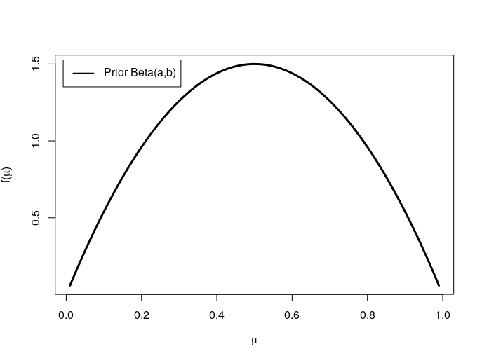
The prior distribution can be visualized with

plot(mu,dbeta(mu,a,b),type="l",lwd = 3,
     col="black",xlab = expression(mu),
     ylab = expression(paste('f(', mu, ')')))

legend('topleft', inset = .02,
     legend = expression(paste("Prior Beta(a,b)")),
     col = c('black'), lwd = 2)

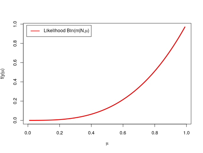
The likelihood can be visualized with

plot(mu,dbinom(N,m,mu),type="l",lwd = 3,
     col="red",xlab = expression(mu),
     ylab = expression(paste('f(y|', mu, ')')))

legend('topleft', inset = .02,
       legend = expression(paste("Likelihood Bin(m|N,",mu,")")),
       col = c('red'), lwd = 2)

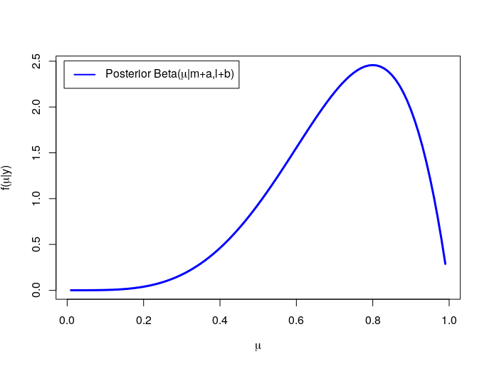
Finally, the posterior is

plot(mu,dbeta(mu,N+a,N-m+b),type="l",lwd = 3,
     col="blue",xlab = expression(mu),
     ylab = expression(paste('f(', mu, '|y)')))

legend('topleft', inset = .02,
       legend = expression(paste("Posterior Beta(",mu,"|m+a,l+b)")),
       col = c('blue'), lwd = 2)

Poisson-Gamma Model

The last example is Poissan likelihood, Gamma prior. Poisson distribution is defined as for \(x_i \sim Poisson(\lambda)\)

\[p(x) \overset{def}{=} \frac{\lambda^x \exp(-\lambda}{x!}\]

Then the likelihood takes the form

\[p_{Y \mid \Lambda}(y \mid \lambda) = \prod_{i=1}^n \lambda^{y_i} \cdot \frac{\exp(-\lambda)}{y_i!} \propto \lambda^{n \cdot \bar{y}} \cdot \exp(-n\lambda)\]

And prior for parameter \(\lambda\) is Gamma distribution \(\lambda \sim \Gamma(a,b)\) which is defined as

\[p(\lambda) \overset{def}{=} \frac{b^a}{\Gamma(a)} \cdot \lambda^{a-1} \cdot \exp(-b\lambda) \propto \lambda^{a-1} \cdot \exp(-b\lambda)\]

Then the posterior is

\[p_{\Lambda \mid Y}(\lambda \mid y) \propto p_{Y \mid \Lambda}(y \mid \lambda) \cdot p_{\Lambda}(\lambda)\] \[\propto \lambda^{n \cdot \bar{y}} \cdot \exp(-n\lambda) \cdot \lambda^{a-1} \cdot \exp(-b\lambda)\] \[\propto \lambda^{a+n \cdot \bar{y} - 1} \cdot \exp(-(b+n)\lambda)\]

Now our posterior is \(\theta \mid y \sim \Gamma(a+\sum y_i, b+n)\). Recall that the expected value of random variable \(\lambda\) in conditions of Gamma distribution is \(\mathop{\mathbb{E}}[\mu] = \frac{a}{b}\), then the posterior mean is \(\mathop{\mathbb{E}}[\mu]=\frac{a+\sum y_i}{a+b+n+\sum y_i}\)

Let’s examine this posterior mean. We can decompose this equality,

\[\mathop{\mathbb{E}}[\mu]=\frac{b}{b+n} \cdot \underbrace{\frac{a}{b}}_{\text{prior mean}} + \frac{n}{b+n} \cdot \underbrace{\frac{\sum y_i}{n}}_{\text{data mean}}\]

This is the wighted average of the prior mean and the data mean! This means, if we choose our \(b\) relatively high, then our posterior contains more information about our prior than likelihood. We call \(b\) effective sample size.

Predictive Distribution

Distribution of the new observations given the observed data is called a posterior predictive distribution. It can be written in the integral for new set of observation \(\hat{Y}\)

\[p_{\hat{Y} \mid Y}(\hat{y} \mid y) = \int_\Theta p_{\hat{Y} \mid \Theta}(\hat{y} \mid \theta) \cdot p_{\Theta \mid Y}(\theta \mid y) d\theta\]

The integrand in the formula is a product of the sampling distribution for the new observations given the parameter, and the posterior distribution of the parameter given the old observations.

Let’s see what is the posterior predictive distribution for one new observation \(\hat{y_1}\) for our Poisson-Gamma model. Define \(a_1 = a + n \cdot \bar{y}\) and \(b_1 = b + n\). The posterior predictive distribution is

\[p_{\hat{Y} \mid Y}(\hat{y_1} \mid y) = \int_\Lambda p_{\hat{Y} \mid \Lambda}(\hat{y} \mid \lambda) \cdot p_{\Lambda \mid Y}(\lambda \mid y) d\lambda\] \[= \int_0^\infty \lambda^{\hat{y_1}} \cdot \frac{\exp(-\lambda)}{\hat{y_1}!} \cdot \frac{b_1^{a_1}}{\Gamma(a_1)} \cdot \lambda^{a_1 - 1} \cdot \exp(-b_1\lambda) d\lambda\] \[= \frac{b_1^{a_1}}{\Gamma(a_1) \cdot \hat{y_1}} \int_0^\infty \lambda^{\hat{y_1} + a_1 -1} \cdot \exp(-(b_1 + 1)\cdot \lambda) d\lambda\]

Define \(t=(b_1+1) \cdot \lambda\), then the equation follows \(\lambda = \frac{t}{b_1 + 1}\). Making this function as differentiable: \(g(t) = \frac{t}{b_1 + 1} \rightarrow d\lambda \frac{1}{b_1 + 1} dt\)

Continue from the last integral,

\[\int_0^\infty \lambda^{\hat{y_1} + a_1 - 1} \cdot \exp(-(b_1 + 1)\lambda) d\lambda\] \[= \int_0^\infty \left(\frac{t}{b_1 + 1}\right)^{\hat{y_1} + a_1 - 1} \cdot \exp(-t) \cdot \frac{1}{b_1 + 1} dt\] \[= \left(\frac{1}{b_1 + 1}\right)^{\hat{y_1} + a_1} \cdot \int_0^\infty t^{\hat{y_1} + a_1 -1} \cdot \exp(-t) dt\] \[= \left(\frac{1}{b_1 + 1}\right)^{\hat{y_1} + a_1} \cdot \Gamma(\hat{y_1}+a_1)\]

Then,

\[p_{\hat{Y} \mid Y}(\hat{y_1} \mid y) = \frac{b_1^{a_1}}{\Gamma(a_1) \cdot \hat{y_1}!} \cdot \left(\frac{1}{b_1 + 1}\right)^{\hat{y_1} + a_1} \cdot \Gamma(\hat{y_1}+a_1)\] \[= \frac{\Gamma(\hat{y_1} + a_1)}{\Gamma(a_1) \cdot \hat{y_1}!} \left(\frac{1}{b_1 + 1}\right)^{\hat{y_1}} \cdot \left(\frac{b_1}{b_1 + 1}\right)^{a_1}\] \[= \frac{\Gamma(\hat{y_1} + a_1)}{\Gamma(a_1) \cdot \hat{y_1}!} \left(1 - \frac{b_1}{b_1 + 1}\right)^{\hat{y_1}} \cdot \left(\frac{b_1}{b_1 + 1}\right)^{a_1} \;\;\; (1)\]

Remember the Negative-Binomial distribution from your basic statistics and probability course at school:

\[p(y) = C(r+y-1,y) \cdot p^r \cdot (1-p)^{y}\]

Where

\[C(r+y-1,y) = \frac{(r+y-1) \cdot (r+y-2) \cdot ... \cdot r}{y!} = \frac{\Gamma(r+y)}{\Gamma(r) \cdot y!}\]

So the equation takes the form \(Neg-Bin(a_1, \frac{b_1}{b_1 + 1})\) and,

\[\hat{y_1} \mid y \sim Neg-Bin(a_1, \frac{b_1}{b_1 + 1})\]

Other Conjugate Pairs

There are other conjugate priors; for example: Normal likelihood + Inverse Gamma prior, Normal likelihood + Scaled inverse chi-squared prior, Uniform likelihood + Pareto prior, Gamma likelihood + Gamma prior etc.

Appendix I: Proof Of Beta Distribution Has Normalizing Term That Gives The Range [0,1]

\[Beta(\mu \mid a,b) = \frac{\Gamma(a+b)}{\Gamma(a) \cdot \Gamma(b)} \mu^{a-1} \cdot (1 - \mu)^{b-1}\] \[\Gamma(a) \cdot \Gamma(b) = \int_0^\infty x^{a-1} \cdot e^{-x} \cdot dx \cdot \int_0^\infty x^{b-1} \cdot e^{-x} \cdot dx\] \[= \int_0^\infty x^{a-1} \cdot e^{-x} \cdot dx \cdot \int_0^\infty y^{b-1} \cdot e^{-y} \cdot dy\] \[= \int_0^\infty \int_0^\infty x^{a-1} \cdot e^{-x} \cdot y^{b-1} \cdot e^{-y} \cdot dx \; dy\] \[t=x+y \rightarrow dt = dx, \;\; dt=dy\] \[= \int_0^\infty \int_0^\infty e^{-t} \cdot x^{a-1} \cdot (t-x)^{b-1} dx dt\] \[= \int_0^\infty e^{-t} \cdot \left(\int_0^t x^{a-1} \cdot (t-x)^{b-1} dx\right) dt \xrightarrow{x=\mu \cdot t}\] \[= \int_0^\infty e^{-t} \cdot \left( t^{a+b-1} \cdot \int_0^t \mu^{a-1} \cdot (1-\mu)^{b-1} d\mu \right) dt\] \[= \int_0^1 e^{-t} \cdot t^{a+b-1} \cdot dt \cdot \int_0^t \mu^{a-1} \cdot (1-\mu)^{b-1} d\mu\] \[= \Gamma(a+b) \cdot \underbrace{\int_0^1 \mu^{a-1} \cdot (1-\mu)^{b-1} d\mu}_{\text{normalizing term}}\]

Notes

Please warn me in the comment section if I did something wrong with mathematics.

References

• Wilks, Daniel S. Bayesian Inference, 2019, Statistical Methods in the Atmospheric Sciences.

• Bishop, Christopher M. Pattern Recognition and Machine Learning, 2006, Springer-Verlag.

• Baron, Michael. Probability and Statistics for Computer Scientists, Second Edition. 2013, hapman & Hall/CRC

• University of California Santa Cruz. Bayesian Statistics: From Concept to Data Analysis. Coursera.

• Barber, David. Bayesian Reasoning and Machine Learning, 2012. Cambridge University Press.

• Conjugate prior. Wikipedia. URL: https://en.wikipedia.org/wiki/Conjugate_prior

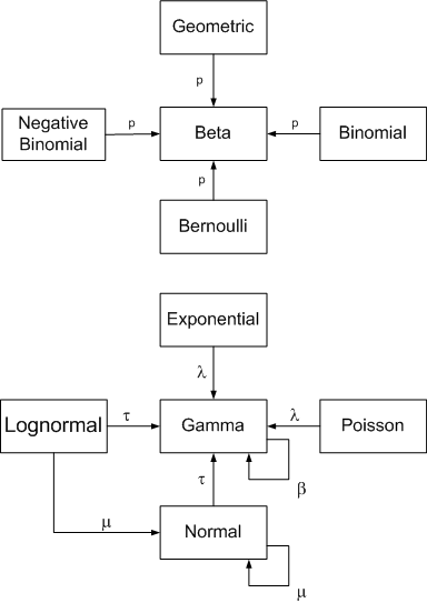
• John D. Cook. Conjugate prior relationships, URL: https://www.johndcook.com/blog/conjugate_prior_diagram/ (last image source)

• Daniel Fink, A Compendium of Conjugate Priors. Environmental Statistics Group, Department of Biology Montana State Univeristy. 1997

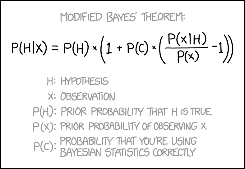
• Modified Bayes’ Theorem, xkcd. A webcomic of romance, sarcasm, math, and language. URL: https://xkcd.com/2059/ (thumbnail source)