
Problem of Unidirectional Models
Throughout the vanishing and exploding gradient problems and long-term dependencies of traditional Recurrent Neural Networks, yet there is an another problem for traditional Recurrent Networks. The characteristics of a sequential data could be unidirectional or bidirectional. Lack of traditional Recurrent Neural Networks is that the state at a particular time unit only has knowledge about the past inputs up to a certain point in a sequential data, but it has no knowledge about future states. What do I mean when I said unidirectional or bidirectional features of a sequential data?
In certain applications like language modelling, the results are vastly improved with knowledge about both past and future states. Let’s give a very simple example based on a very simple sentence: “The rat ate cheese”.
Figure 1: Phrase tree of “The rat ate cheese.”
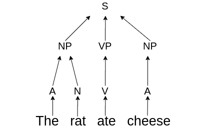
The word “rat” and the word “cheese” are related in someway. There is a ‘passive’ advatage in using knowledge about both the past and future words. Cheese is generally eaten by rats and rats generally eat cheese. As I said this is a very simple example.
The Architecture of Bidirectional Recurrent Neural Networks
In the bidirectional Recurrent Neural Networks, we have seperate hidden states/layers \(h_t\) and \(h_t'\) for the forward and backward directions. The forward hidden states interact with each other and the same is true for the backward hidden states. There is no multilayered connections between them. However, both \(h_t\) and \(h_t'\) receive input from the same vector \(x_t\) and they interact with same output vector \(\hat{y}_t\). Here is a very good visual comparsion (images are taken from colah’s blog) between traditional Recurrent Neural Networks and bidirectional Recurrent Neural Networks:
Figure 2: Traditional Recurrent Neural Networks.
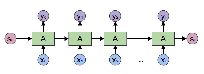
Figure 3: Bidirectional Recurrent Neural Networks.
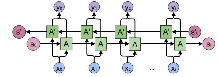
In general, any property of the current word can be predicted more effectively using this approach, because it uses the context on both sides. For example, the ordering of words in several languages is somewhat different depending on grammatical structure. Bidirectional Recurrent Neural Networks work well in tasks where the predictions are based on bidirectional context like handwrittings.
Forward Propagation Over Directions
Before we go for forward propagation equations, it is easier to understand the structure of equations with a simple computational graph.
Figure 4: Computational graph for 3 layered Bidirectional RNN.
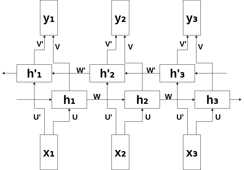
Backward layers and weights are shown with a single apostrophe. To make a simpler representation, bias units are not shown.
The forward propagation is similiar with traditional Recurrent Networks. The only difference is there are two equations for backward units and forward units.
\[h_t = tanh(U x_t + W h_{t-1})\] \[h_t' = tanh(U' x_t + W' h_{t+1}')\] \[\hat{y}_t = softmax(V h_t + V' h_t')\]It is easy to see that the bidirectional equations are simple generalizations of the conditions used in a single direction. It is assumed that there are a total \(T\) time-stamps in the neural network shown above, where \(T\) is the length of the squence. One question is about the forward input at the boundary conditions corresponding to \(t=1\) and the backward input at \(t=T\), which are not defined. In such cases, one can use a default constant value of 0.5 in each case, although one can also make the determination of these values as a part of the learning process.
An important property of this forward process, the hidden states of forward direction and backward direction do not interract with one another at all. So, in the learning process, one can first run the forward propagation for the forward direction to compute hidden states and then run the forward propagation for the backward direction to compute hidden states. After that, the output states are computed from the hidden states in the two directions. Also, one can compute forward propagations with parallelization.
Gradients Over Directions
We shown the generalized forward propagations above. Not it is time to compute gradients over weights. First, the partial derivatives are computed with respect to the output states due to both forward and backward states point to the output nodes. (the subscripts of subscripts are just for “dummy indexing”.)
Loss is to be the cross-entropy loss:
\[\mathop{\mathbb{E_t}}[y_{t_i},\hat{y}_{t_i}] = -y_{t_i} log \hat{y}_{t_i}\] \[\mathop{\mathbb{E_t}}[y_t,\hat{y}_t] = -y_{t}\; log \; \hat{y}_{t}\]Then the loss is,
\[L(y,\hat{y}) = -\frac{1}{N}\sum_{t}^{T}y_t \;log\; \hat{y}_y\]- Now let’s calculate the gradients for \(V\):
It is more clear for derivatives with denoting \(q_t = V h_t + V' h_t'\):
\[\frac{\partial E_t}{\partial V_{ij}} = \frac{\partial E_t}{\partial \hat{y}_{t_k}} \frac{\hat{y}_{t_k}}{\partial q_{t_l}} \frac{\partial q_{t_l}}{\partial V_{ij}}\]You can clearly see that for \(E_t = -y_{t_k}\;log\;\hat{y}_{t_k}\), the derivative is (1)
\[\frac{\partial E_t}{\partial \hat{y}_{t_k}} = -\frac{y_{t_k}}{\hat{y}_{t_k}}\]Now, we will derive \(\hat{y}_{t_k} = softmax(q_{t_l})\), which is \(\frac{\partial \hat{y}_{t_k}}{\partial q_{t_l}}\). But, firstly, we have to evaluate the derivation of softmax function.
\[\hat{y}_{t_k} = \frac{\exp(q_{t_k})}{\sum_{n}^{N}\exp(q_{t_n})}\]so softmax is a \(\mathbb{R}^n \rightarrow \mathbb{R}^n\) mapping function:
\[\hat{y}_{t_k}: \begin{bmatrix} q_{t_1} \\ q_{t_2} \\ q_{t_3}\\ \vdots\\ q_{t_N} \end{bmatrix} \rightarrow \begin{bmatrix} \hat{y}_{t_1} \\ \hat{y}_{t_2} \\ \hat{y}_{t_3}\\ \vdots\\ \hat{y}_{t_N} \end{bmatrix}\]Therefore, the Jacobian of the softmax will be:
\[\frac{\partial \hat{y}_{t}}{\partial q_{t}} = \begin{bmatrix} \frac{\partial \hat{y}_{t_1}}{\partial q_{t_1}} & \frac{\partial \hat{y}_{t_1}}{\partial q_{t_2}} & \cdots & \frac{\partial \hat{y}_{t_1}}{\partial q_{t_N}}\\ \frac{\partial \hat{y}_{t_2}}{\partial q_{t_1}} & \frac{\partial \hat{y}_{t_2}}{\partial q_{t_2}} & \cdots & \frac{\partial \hat{y}_{t_2}}{\partial q_{t_N}}\\ \vdots & \vdots & \cdots & \vdots \\ \frac{\partial \hat{y}_{t_N}}{\partial q_{t_1}} & \frac{\partial \hat{y}_{t_N}}{\partial q_{t_2}} & \cdots & \frac{\partial \hat{y}_{t_N}}{\partial q_{t_N}} \end{bmatrix}\]Let’s compute the \(\frac{\partial \hat{y}_{t_k}}{\partial q_{t_l}}\):
\[\frac{\partial \hat{y}_{t_k}}{\partial q_{t_l}} = \frac{\partial}{\partial q_{t_l}} \frac{\exp(q_{t_k})}{\sum_{n}^{N} \exp(q_{t_n})}\]You all remember the quotient rule for derivatives from high school; for \(f(x) = \frac{g(x)}{h(x)}\), the derivative of \(f(x)\) is given by:
\[f'(x) = \frac{g'(x) h(x) - h'(x) g(x)}{h^2(x)}\]So, in our case, \(g_k = \exp(q_{t_k})\) and \(h_k = \sum_{n}^{N}\exp(q_{t_n})\). NO matter what the derivative \(\frac{\partial}{\partial q_{t_l}} h_k = \frac{\partial}{\partial q_{t_l}} \sum_{n}^{N}\exp(q_{t_n})\) is equal to \(\exp(q_{t_l})\) because \(\frac{\partial}{\partial q_{t_l}} \exp(q_{t_n}) = 0\) for \(l \neq n\).
Derivative of \(g_k\) respect to \(q_{t_l}\) is \(\exp(q_{t_l})\) only if \(k=l\), otherwise it is a constant 0. Therefore, if we derive the gradient of the off-diagonal entries of the Jacobian will yield:
\[\frac{\partial}{\partial q_{t_l}} \frac{\exp(q_{t_k})}{\sum_{n}^{N}\exp(q_{t_n})} = \frac{0 \sum_{n}^{N}\exp(q_{t_n}) - \exp(q_{t_l}) \exp(q_{t_k})}{\left[\sum_{n}^{N}\exp(q_{t_n}\right]^2}\] \[\;\;\;\;= - \frac{\exp(q_{t_l})}{\sum_{n}^{N}\exp(q_{t_n})} \frac{\exp(q_{t_k})}{\sum_{n}^{N}\exp(q_{t_n})}\] \[\;\;\;\; = -\hat{y}_{t_k} \hat{y}_{t_l}\]Similiarly, derive the gradient of \(diag(\partial \hat{y}_k / \partial q_l)\) for \(k=l\), we have that:
\[\frac{\partial}{\partial q_{t_l}} \frac{\exp(q_{t_k})}{\sum_{n}^{N}\exp(q_{t_n})} = \frac{\exp(q_{t_k}) \sum_{n}^{N}\exp(q_{t_n}) - \exp(q_{t_l}+q_{t_k})}{\left[\sum_{n}^{N}\exp(q_{t_n})\right]^2}\] \[\;\; = \frac{\exp(q_{t_k})\left(\sum_{n}^{N} \exp(q_{t_n}) - \exp(q_{t_l})\right)}{\left[\sum_{n}^{N}\exp(q_{t_n})\right]^2}\] \[\;\;\;\; = \hat{y}_{t_k} (1-\hat{y}_{t_l})\]So ve have (2)…
\[\frac{\partial \hat{y}_{t_k}}{\partial q_{t_l}}= \begin{cases} -\hat{y}_{t_k} \hat{y}_{t_l},& \text{if } k \neq l\\ \hat{y}_{t_k} (1-\hat{y}_{t_l}), & \text{if } k = l \end{cases}\]If we put (1) and (2) together, gives us a sum over all values of \(k\) to obtain \(\frac{\partial E_t}{\partial q_{t_l}} =\)
\[- \frac{y_{t_l}}{\hat{y}_{t_l}} \hat{y}_{t_l} + \sum_{k \neq l} \left(\frac{y_{t_k}}{\hat{y}_{t_k}} \right) (-\hat{y}_{t_k} \hat{y}_{t_l}\] \[= -y_{t_l} + y_{t_l} \hat{y}_{t_l} + \sum_{k \neq l} y_{t_k} \hat{y}_{t_l}\] \[= -y_{t_l} + \hat{y}_{t_l} \sum_{k} y_{t_k}\]If you recall that \(y_t\) are all one-hot vectors, then that sum is just equal to 1. So we have (3),
\[\frac{\partial E_t}{\partial q_{t_l}} = \hat{y}_{t_l} - y_{t_l}\]Recall that we defined \(q_t = V h_t + V h_t'\), so for dummy indexing, we can say \(q_{t_l} = V_{lm} h_{t_m} + V_{lm}' h_{t_m}'\). Then we have (4),
\[\frac{\partial q_{t_l}}{\partial V_{ij}} = \frac{\partial}{\partial V_{ij}} (V_{lm} h_{t_m} + V_{lm}' h_{t_m}')\] \[\;\; = \frac{\partial}{\partial V_{ij}} (V_{lm} h_{t_m})\] \[= \delta_{il} \delta_{jm} h_{t_m}\] \[= \delta_{il} h_{t_j}\]To combining our results we obtain (5):
\[\frac{\partial E}{\partial V} = (\hat{y}_t - y_y) \otimes h_t\]- Now let’s calculate the gradients for \(W\):
It is clear that \(\hat{y}_{t}\) depends on \(W\) both directly and indirectly. We can directly see the partial derivatives like:
\[\frac{\partial E_t}{\partial W{ij}} = \frac{\partial E_t}{\partial \hat{y}_{t_k}} \frac{\partial \hat{y}_{t_k}}{\partial q_{t_l}} \frac{\partial q_{t_l}}{\partial h_{t_m}} \frac{\partial h_{t_m}}{\partial W{ij}}\]Yes this is the partial derivatives respect to \(W{ij}\) but note that at the last term, there is an implicit dependency of \(h_t\) on \(W{ij}\) through \(h_{t_1}\). Hence, we have
\[\frac{\partial h_{t_m}}{\partial W_{ij}} \longrightarrow \frac{\partial h_{t_m}}{\partial W_{ij}} + \frac{\partial h_{t_m}}{\partial h_{t-1_n}} \frac{\partial h_{t-1_n}}{\partial W_{ij}}\]We can apply this again and again (6):
\[\frac{\partial h_{t_m}}{\partial W_{ij}} \longrightarrow \frac{\partial h_{t_m}}{\partial W_{ij}} + \frac{\partial h_{t_m}}{\partial h_{t-1_n}} \frac{\partial h_{t-1_n}}{\partial W_{ij}} + \frac{\partial h_{t_m}}{\partial h_{t-1_n}} \frac{\partial h_{t-1_n}}{\partial h_{t-2_p}} \frac{\partial h_{t-2_p}}{\partial W_{ij}}\]This equation continues until \(h_{-1}\) is reached. \(h_{-1}\) is a vector of zeros.
Note that of these four terms we have already calculated first two derivatives.
The third one is:
\[\frac{\partial q_{t_l}}{\partial h_{t_m}} = \frac{\partial}{\partial h_{t_m}} (V_{lb} h_{t_b} + V_{lb}' h_{t_b}')\] \[\;\;=\frac{\partial}{\partial h_{t_m}} (V_{lb} h_{t_b})\] \[= V_{lb} \delta_{bm}\] \[= V_{lm}\]The last term in (6) collapses to \(\frac{\partial h_{t_m}}{\partial h_{t-2_n}} \frac{h_{t-2_n}}{\partial W_{ij}}\) and we can turn the first item into \(\frac{\partial h_{t_m}}{\partial h_{t_n}} \frac{\partial h_{t_n}}{\partial W_{ij}}\). Then we have the compact form that is:
\[\frac{\partial h_{t_m}}{\partial W_{ij}} = \frac{\partial h_{t_m}}{\partial h_{x_n}} \frac{\partial h_{x_n}}{\partial W_{ij}}\]And we rewrite this as sum over all values of \(x\) less than \(t\), we have (7):
\[\frac{\partial h_{t_m}}{\partial W_{ij}} = \sum_{x=0}^{t} \frac{\partial h_{t_m}}{\partial h_{x_n}} \frac{\partial h_{x_n}}{\partial W_{ij}}\]And, combining all:
\[\frac{\partial E_t}{\partial W_{ij}} = (\hat{y}_{t_l} - y_{t_l}) V_{lm} \sum_{x=0}^{t} \frac{\partial h_{t_m}}{\partial h_{x_n}} \frac{\partial h_{x_n}}{\partial W_{ij}}\]- Now let’s calculate the gradients for \(U\):
It is similiar to calculating the gradient for \(U\):
\[\frac{\partial E_t}{\partial U_{ij}} = \frac{\partial E_t}{\partial \hat{y}_{t_k}} \frac{\partial \hat{y}_{t_k}}{\partial q_{t_l}} \frac{\partial q_{t_l}}{\partial h_{t_m}} \frac{\partial h_{t_m}}{\partial U_{ij}}\] \[\frac{\partial h_{t_m}}{\partial U_{ij}} = \sum_{x=0}^{t} \frac{\partial h_{t_m}}{\partial h_{x_n}} \frac{\partial h_{x_n}}{\partial U_{ij}}\]Then we have, \(\frac{\partial E_t}{\partial U_{ij}} = (\hat{y}_{t_l} - y_{t_l}) V_{lm} \sum_{x=0}^{t} \frac{\partial h_{t_m}}{\partial h_{x_n}} \frac{\partial h_{x_n}}{\partial U_{ij}}\)
Backward Gradients
Backpropagation through time over backward direction is the same as the forward direction. It is useless to rewrite the same equations. Check partial derivatives for \(V', W'\) and \(U'\) yourself.
Results
To serve up these steps:
- Compute forward and backwards hidden states in independent and separate passes.
- Compute output states from backwards and forward hidden states.
- Compute partial derivatives of loss with respect to output states and each copy of the output parameters.
- Compute partial derivatives of loss with respect to forward states and backward states INDEPENDENTLY using backpropagation algorithm. Use these computations to evaulate partial derivatives with respect to each copy of the forwards and backwards parameters.
- Aggregate partial derivatives over shared parameters.
References
- Neural Networks and Deep Learning, Charu C. Aggarwal, Springer International Publishing, ISBN 978-3-319-94463-0
- BPTT post of Denny Britz
- Figure 2 and Figure 3 from colah’s blog

Leave a comment