Language And Representation

“Every choice of phrasing and spelling and tone and timing carries countless signals and contexts and subtexts and more… and every listener interprets those signals in their own way. Language isn’t a formal system. Language is glorious chaos.”

Words and meanings are ambigious. ~85% of words are unambigious, however, accounting for only ~15% of the vocabulary, are very common words, and hence ~55% of word tokens in running text are ambigious [1]:

• earnings growth took a back/JJ seat
• a small building in the back/NN
• a clear majority of senators back/VBP at bill
• Dave began to back/VB toward the door
• enable the country to buy back/RP about debt
• I was twenty-one back/RB then

Even though many words are easy to disambiguate linguistically, it is not always easy to represent this words computationally. Grammar is a mental system, a cognitive part of the brain/mind, which, if it is one’s first native language, is acquired as a child without any specific instruction. Children develop language rapidly and efficiently, that is, with relatively few errors, because the basic form of language is given to them by human biology (the logical problem of language acquisition, Noam Chomsky, 1955) [2]. So, imagine that how hard it is to represent well while we have ambiguity in our brain’s understanding. In this post, I will introduce and compare a comprehensive typology of word representation models.

Frequency Matrices

The most simple yet efficient method of representing words is, as traditionally, term-document matrix. It is basically a frequency matrix of “how many times has this word been in this document”. For example, term-document matrix for some of Shakespeare’s play.

…	As You Like It	Twelfth Night	Julius Caesar	Henry V
battle	1	0	7	13
god	114	80	62	89
fool	36	58	1	4
wit	20	15	2	3

The dimensionality of this matrix is \(\mid V \mid \times \mid d \mid\), where \(\mid V \mid\) is our vocabulary length and \(\mid d \mid\) is document number. With this approach, the document “Julius Caesar” can be represented with [7, 62, 1, 2, …] with dimensionality \(\mid V \mid\). Also words can be represented with term-document matrix: the word “battle” can be represented with [1, 0, 7, 13, …] with dimensionality \(\mid d \mid\).

Also, word-word co-occurence matrix can be used for representing words. It is basically a frequency matrix of “how many times has this word been with this word, in some context”.

…	aardvark	…	computer	data	sugar
cherry	0	…	2	8	25
strawberry	0	…	0	0	19
fool	0	…	1670	1683	4
information	0	…	3325	3982	13

The dimensionality of this matrix is \(\mid V \mid \times \mid V \mid\). With this approach, the word “cherry” can be represented with [0, …, 2, 8, 25] with dimensionality \(\mid V \mid\). This approach still gives acceptable good analogies with cosine similarity. Cosine similarity is normalized dot product between two word vectors:

\[\text{cosine-sim}(\vec{w_1},\vec{w_2}) = \frac{\vec{w_1} \cdot \vec{w_2}}{\lVert \vec{w_1} \rVert \lVert \vec{w_2} \rVert}\]

It ranges from 1 to -1. Orthogonal vectors (not similar) gives 0.

TF-IDF

TF-IDF is just a weighing method for co-occurence matrix. Words that occur nearby frequently (pie nearby cherry) are more important than words that only appear once or twice. Yet words that are too frequent (the, good, that etc.) are unimportant. TF-IDF captures that information. The term frequency (tf) is defined as the frequency of the word \(w\) in the document \(d\):

\[\text{tf}_{w,d} = \text{count}(w, d)\]

and the inverse document frequency (idf) is defined as

\[\text{idf}_{w} = \log_{10} \left( \frac{N}{\text{df}_w} \right)\]

where \(N\) is the total number of documents, \(\text{df}_w\) is is the total number of documents that includes \(w\). Soi the TF-IDF weighted value for word \(w\) is defined as

\[w_d = \text{tf}_{w,d} \times \text{idf}_{w}\]

Positive Pointwise Mutual Information (PPMI)

Positive Pointwise Mutual Information (PPMI) is an alternative for TF-IDF model. It is defined as

\[\text{PPMI}(w, c) = \max\left(\log_2\frac{p(w,c)}{p(w)\cdot p(c)}, 0\right)\]

Assume that we have a co-occurence matrix \(CO\) with \(\mid V \mid\) rows (words), \(C\) columns (contexts). \(CO_{i,j}\) is “number of times word \(w_i\) occurs in context \(c_j\). So,

\[p(w_i,c_j) = \frac{CO_{i,j}}{\sum_{i=1}^{\mid V \mid} \sum_{j=1}^{C} CO_{i,j}}\] \[p(w_i) = \frac{\sum_{j=1}^{C} CO_{i,j}}{\sum_{i=1}^{\mid V \mid} \sum_{j=1}^{C} CO_{i,j}}\] \[p(c_j) = \frac{\sum_{i=1}^{\mid V \mid}CO_{i,j}}{\sum_{i=1}^{\mid V \mid} \sum_{j=1}^{C} CO_{i,j}}\]

Singular Value Decomposition

Singular Value Decomposition (SVD) is a central matrix decomposition technique in linear algebra. The problem of PPMI and TF-IDF vectors are sparsity. They have too many zero values. Like SVD, Matrix factorization techniques also give good vector representations. In Linear Algebra, any rectangular matrix can be decomposed into three matrices

\[\small \begin{bmatrix} X \end{bmatrix}_{\in \mathbb{R}^{\mid V \mid \times \mid V \mid}} = \begin{bmatrix} W \end{bmatrix}_{\in \mathbb{R}^{\mid V \mid \times \mid V \mid}} \begin{bmatrix} \sigma_1 & \cdots & 0 \\ \vdots & \ddots & \vdots\\ 0 &\cdots & \sigma_V \end{bmatrix}_{\in \mathbb{R}^{\mid V \mid \times \mid V \mid}} \begin{bmatrix} C \end{bmatrix}_{\in \mathbb{R}^{\mid V \mid \times \mid V\mid}}\]

So, our goal is now to create more sophisticated good word vectors, suppose that \(X\) is our word-word co-occurence matrix. We can get good vector representations by factorizing this matrix, or reducing the dimensionality. It allows us to represent our vectors more densely in lower cost memory.

\[\small \begin{bmatrix} X \end{bmatrix}_{\in \mathbb{R}^{\mid V \mid \times \mid V \mid}} = \begin{bmatrix} W \end{bmatrix}_{\in \mathbb{R}^{\mid V \mid \times k}} \begin{bmatrix} \sigma_1 & \cdots & 0 \\ \vdots & \ddots & \vdots\\ 0 &\cdots & \sigma_k \end{bmatrix}_{\in \mathbb{R}^{k \times k}} \begin{bmatrix} C \end{bmatrix}_{\in \mathbb{R}^{k \times \mid V\mid}}\]

The matrix \(W\) tells us how to map our input sparse feature vectors into these k-dimensional dense feature vectors. SVD (and other factorization methods) had an good role on comparisons. For example, in GloVe: Global Vectors for Word Representation, authors compared their novel model with Singular Value Decomposition as a baseline.

Distributional Hypothesis

Suppose that we have a set \(E = \{e_{w_i}: w_i \in V\}\). This is a set of our word representations. Say that, those representations are a collection of vectors, that are dense. What are the dimensions of these vectors? Take a look word “queen”. Since the word “queen” means “the female ruler of an independent state”, should it has a dimension that represents “royality” or “gender”? Or, the word “teeth”, should it has a dimension that represents “plurality”? Maybe we should define more common dimensions. For example, words can have affective meanings [1]. Osgood et al. 1957, proposed that words varied along three important dimensions of affective meaning: valence, arousal, dominance:

• valence: the pleasantness of the stimulus.

• arousal: the intensity of emotion provoked by the stimulus.

• dominance: the degree of control exerted by the stimulus.

For instance, the word “delighted” has high valence while the word “upset” does not. Or, the word “thrilling” has high arousal while the word “serene” does not. More examples can be given. Actually, we don’t know exactly what are the dimensions of those vector. Now, our question is “how to get them” or “how can we learn those word vectors”. The discipline called Distributional Hypothesis plays a big role here. Distributional Hypothesis is mainly introduced by John Rupert Firth in 1957. It basically says, words with similar distributions have similar meanings. Words that occur in similar contexts tend to have similar meanings. The link between similarity and words are distributed and similarity in what they mean is called distributional hypothesis or distributional semantics in the field of Computational Linguistics [1]. So what can be counted when we say similar contexts? For example if you surf on the Wikipedia page of Johann Sebastian Bach, the words in this page somehow related with each other in the context of Bach. Or maybe an essay about Johann Sebastian Bach, suppose that you don’t know the exact meaning of the word “composer”, but you know that Bach is an classical musician and writes music pieces. While reading this essay, you will encounter the word “composer” so many times: “Johann Sebastian Bach is the smartest composer of Baroque period”. Then your brain does some kind of acquisition: “Bach writes music and the paragraph says, Bach is a composer. Then the meaning of composer would be the person who writes music. But what is Baroque? The word period comes after Baroque. So Baroque is some kind of period and related with Bach in a comparison way. So Baroque is a historical period that is related with classical music”. And, this is the Distributional Hypothesis. But where are the vectors and dimensions?

word2vec

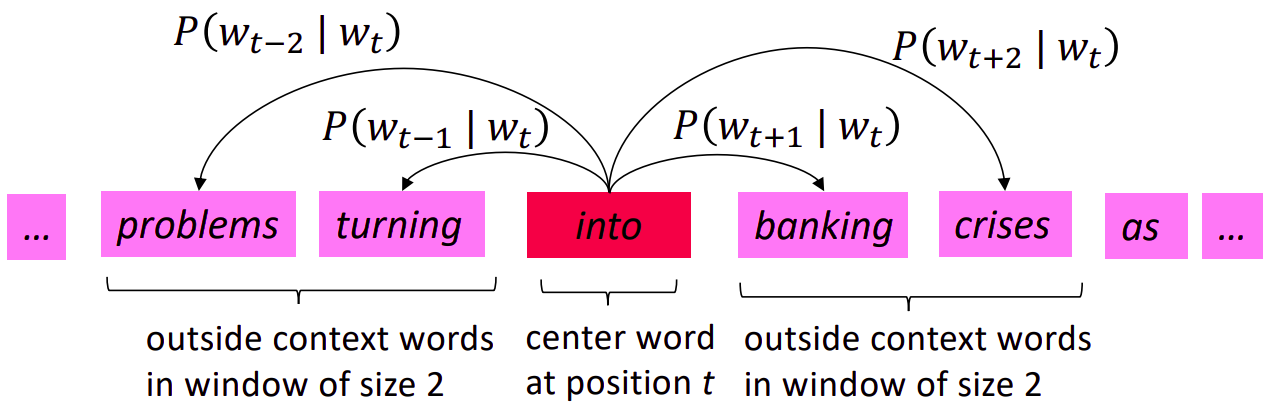
word2vec is a word representation algorithm, proposed in the paper called Distributed Representations of Words and Phrases and their Compositionality (Mikolov et al., 2013). It allows you to learn the high-quality distributed vector representations that capture a large number of precise syntactic and semantic word relationships [3]. word2vec algorithm uses skip-gram Efficient Estimation of Word Representations in Vector Space model to learn efficient vector representations. Those learned word vectors has interesting property, words with semantic and syntactic affinities give the necessary result in mathematical similarity operations. Suppose that you have a sliding window of a fixed size moving along a sentence: the word in the middle is the “target” and those on its left and right within the sliding window are the context words. The skip-gram model is used to predict the probabilities of a word being a context word for the given target.

Target - Context pairs 1	Target - Context pairs 2

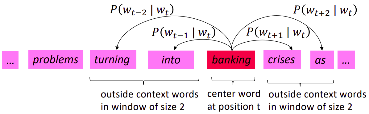image source [5].

For example consider this sentence,

“A change in Quantity also entails a change in Quality”

Our target and context pairs for window size of 5:

Sliding window (size = 5)	Target word	Context
[A change in]	a	change, in
[A change in Quantity ]	change	a, in, quantitiy
[A change in Quantity also]	in	a, change, quantitiy,also
…	…	…
[entails a change in Quality]	change	entails, a, in, Quality
[a change in Quality]	in	a, change, Quality
[change in Quality]	quality	change, in

Each context-target pair is treated as a new observation in the data. For each position \(t=1, ..., T\) predict context words within a window of fixed size \(m\) given center word \(w_j\). In Skip-gram connections we have an objective to maximize, likelihood (or minimize negative log-likelihood):

\[\max \limits_{\theta} \prod_{\text{center}} \prod_{\text{context}} p(\text{context}|\text{center} ;\theta)\] \[= \max \limits_{\theta} \prod_{t=1}^T \prod_{-c \leq j \leq c, j \neq c} p(w_{t+j}|w_t; \theta)\] \[= \min \limits_{\theta} -\frac{1}{T} \prod_{t=1}^T \prod_{-c \leq j \leq c, j \neq c} p(w_{t+j}|w_t; \theta)\] \[= \min \limits_{\theta} -\frac{1}{T} \sum_{t=1}^T \sum_{-c \leq j \leq c, j \neq c} \log p(w_{t+j}|w_t; \theta)\]

So, How can we calculate those probabilities? Softmax gives the normalized probabilities.

\[p(w_c \mid w_t) = \frac{\exp(v_{w_c}^T v_{w_t})}{\sum_{i=0}^{\mid V \mid} \exp(v_{w_i}^T v_{w_t})}\]

maximizing this log-likelihood function under \(v_{w_t}\) gives you the most likely value of the \(v_{w_t}\) given the data.

\[\frac{\partial}{\partial v_{w_t}}\cdot \log \frac{\exp(v_{w_c}^T v_{w_t})}{\sum_{i=0}^{\mid V \mid} \exp(v_{w_i}^T v_{w_t})}\] \[= \frac{\partial}{\partial v_{w_t}}\cdot \log \underbrace{\exp(v_{w_c}^T v_{w_t})}_{\text{numerator}} - \frac{\partial}{\partial v_{w_t}}\cdot \log \underbrace{\sum_{i=0}^{\mid V \mid} \exp(v_{w_i}^T v_{w_t})}_{\text{denominator}}\] \[\frac{\partial}{\partial v_{w_t}} \cdot v_{w_c}^T v_{w_t} = v_{w_c} \; \; (\text{numerator})\]

Now, it is time to derive denominator.

\[\frac{\partial}{\partial v_{w_t}}\cdot \log \sum_{i=0}^{\mid V \mid} \exp(v_{w_i}^T v_{w_t})\] \[= \frac{1}{\sum_{i=0}^{\mid V \mid} \exp(v_{w_i}^T v_{w_t})} \cdot \frac{\partial}{\partial v_{w_t}} \sum_{i=0}^{\mid V \mid} \exp(v_{w_i}^T v_{w_t})\] \[= \frac{1}{\sum_{i=0}^{\mid V \mid} \exp(v_{w_i}^T v_{w_t})} \cdot \sum_{i=0}^{\mid V \mid} \frac{\partial}{\partial v_{w_t}} \cdot \exp(v_{w_i}^T v_{w_t})\] \[= \frac{1}{\sum_{i=0}^{\mid V \mid} \exp(v_{w_i}^T v_{w_t})} \cdot \sum_{i=0}^{\mid V \mid} \exp(v_{w_i}^T v_{w_t}) \frac{\partial}{\partial v_{w_t}} v_{w_i}^T v_{w_t}\] \[= \frac{\sum_{i=0}^{\mid V \mid} \exp(v_{w_i}^T v_{w_t}) \cdot v_{w_i}}{\sum_{i=0}^{\mid V \mid} \exp(v_{w_i}^T v_{w_t})} \;\; (\text{denominator})\]

To sum up,

\[\frac{\partial}{\partial w_t} \log p(w_c \mid w_t) = v_{w_c} - \frac{\sum_{j=0}^{\mid V \mid} \exp(v_{w_j}^T v_{w_t}) \cdot v_{w_j}}{\sum_{i=0}^{\mid V \mid} \exp(v_{w_i}^T v_{w_t})}\] \[= v_{w_c} - \sum_{j=0}^{\mid V \mid} \frac{\exp(v_{w_j}^T v_{w_t})}{\sum_{i=0}^{\mid V \mid} \exp(v_{w_i}^T v_{w_t})} \cdot v_{w_j}\] \[\underbrace{= v_{w_c} - \sum_{j=0}^{\mid V \mid} p(w_j \mid w_t) \cdot v_{w_j}}_{\nabla_{w_t}\log p(w_c \mid w_t)}\]

This is the observed representation subtract \(\mathop{\mathbb{E}}[w_j \mid w_t]\).

Noise Contrastive Estimation

The Noise Contrastive Estimation (NCE) metric intends to differentiate the target word from noise samples using a logistic regression classifier Noise-contrastive estimation: A new estimation principle for unnormalized statistical models, Gutmann et al., 2010. In softmax computation, look at the denominator. The summation over \(\mid V\mid\) is computationally expensive. The training or evaluation takes asymptotically \(O(\mid V \mid)\). In a very large corpora, the most frequent words can easily occur hundreds or millions of times (“in”, “and”, “the”, “a” etc.). Such words provides less information value than the rare words. For example, while the skip-gram model benefits from observing co-occurences of “bach” and “composer”, it benefits much less from observing the frequent co-occurences of “bach” and “the” [3] . For every training step, instead of looping over the entire vocabulary, we can just sample several negative examples! We “sample” from a noise distribution \(P_n(w)\) whose probabilities match the ordering of the frequency of the vocabulary. Consider a pair \((w_t, w_c)\) of word and context. Did this pair come from the training data? Let’s denote by \(p(D=1 \mid w_t,w_c)\) the probability that \((w_t, w_c)\) came from the corpus data. Correspondingly \(p(D=0 \mid w_t,w_c)\) will be the probability that \((w_t, w_c)\) didn’t come from the corpus data [5]. First, let’s model \(p(D=1 \mid w_t,w_c)\) with sigmoid:

\[p(D=1 \mid w_t,w_c) = \sigma(v_{w_c}^T v_{w_t}) = \frac{1}{1 + \exp(- v_{w_c}^T v_{w_t})}\]

Now, we build a new objective function that tries to maximize the probability of a word and context being in the corpus data if it indeed is, and maximize the probability of a word and context not being in the corpus data if it indeed is not. Maximum likelihood says:

\[\small \max \prod_{(w_t, w_c) \in D} p(D=1 \mid w_t,w_c) \times \prod_{(w_t, w_c) \in D'} p(D=0 \mid w_t,w_c)\] \[\small = \max \prod_{(w_t, w_c) \in D} p(D=1 \mid w_t,w_c) \times \prod_{(w_t, w_c) \in D'} 1 - p(D=1 \mid w_t,w_c)\] \[\small = \max \sum_{(w_t, w_c) \in D} \log p(D=1 \mid w_t,w_c) + \sum_{(w_t, w_c) \in D'} \log (1 - p(D=1 \mid w_t,w_c))\] \[\small = \max \sum_{(w_t, w_c) \in D} \log \frac{1}{1 + \exp(- v_{w_c}^T v_{w_t})} + \sum_{(w_t, w_c) \in D'} \log \left(1 - \frac{1}{1 + \exp(- v_{w_c}^T v_{w_t})}\right)\] \[\small = \max \sum_{(w_t, w_c) \in D} \log \frac{1}{1 + \exp(- v_{w_c}^T v_{w_t})} + \sum_{(w_t, w_c) \in D'} \log \frac{1}{1 + \exp(v_{w_c}^T v_{w_t})}\]

Maximizing the likelihood is the same as minimizing the negative log likelihood:

\[\small L = - \sum_{(w_t, w_c) \in D} \log \frac{1}{1 + \exp(- v_{w_c}^T v_{w_t})} - \sum_{(w_t, w_c) \in D'} \log \frac{1}{1 + \exp(v_{w_c}^T v_{w_t})}\]

The Negative Sampling (NEG) proposed in the original word2vec paper. NEG approximates the binary classifier’s output with sigmoid functions as follows:

\[p(d=1 \vert v_{w_c}, v_{w_t}) = \sigma(v_{w_c}^T v_{w_t})\] \[p(d=0 \vert v_{w_c}, v_{w_t}) = 1 - \sigma(v_{w_c}^T v_{w_t}) = \sigma(-v_{w_c}^T v_{w_t})\]

So the objective is

\[L = - [ \log \sigma(v_{w_c}^T v_{w_t}) + \sum_{\substack{i=1 \\ \tilde{w}_i \sim Q}}^K \log \sigma(v_{\tilde{w}_i}^T v_{w_t})]\]

In the above formulation, \({v_{\tilde{w}_i} \mid i = 1 . . . K}\) are sampled from \(P_n(w)\). How to define \(P_n(w)\)? In the word2vec paper \(P_n(w)\) defined as

\[P_n(w_i) = 1 - \sqrt{\frac{t}{freq(w_i)}} \;\; t \approx 10^{-5}\]

This distribution assigns lower probability for lower frequency words, higher probability for higher frequency words. Hence, this distribution is sampled form a unigram distribution \(U(w)\) raised to the \(\frac{3}{4}\)rd power. The unigram distribuiton is defined as

\[P_n(w_i) = \frac{freq(w_i)^\frac{3}{4}}{\sum_{j=0}^M freq(w_j)^\frac{3}{4}}\]

Raising the unigram distribution \(U(w)\) to the power of \(\alpha\) has an effect of smoothing out the distribution. It attempts to combat the imbalance between common words and rare words by decreasing the probability of drawing common words, and increasing the probability drawing rare words.

In the detail, first word vectors are initialized randomly, then updated by their gradient. word2vec gives good vectors representations, it is successful on semantic and syntactic analogies (cosine similarty tasks). For example “woman is to queen as man is to X. In this example X should be the word king. This behaviour can be formulated linearly: vec(“queen”) - vec(“woman”) + vec(“man”) = vec(“king”). Same formulation is valid on syntactic analogies.

GloVe

GloVe GloVe: Global Vectors for Word Representation, Pennington et al., 2014 combines the advantages of global matrix factorization (such as Latent Semantic Analysis) and local context window methods. Methods like skip-gram (word2vec) may do better on the analogy task, but they poorly utilize the statistics of the corpus since they train on separate local context windows instead of on global co-occurence counts. GloVe defines a matrix \(\mathbf{X} = [X_{ij}]\) which represents word-word co-occurence counts. Entries \([X_{ij}]\) tabluate the number of times word \(j\) occurs in the context of word \(i\). If we choose our context-target pairs as in word2vec algorithm, then \(\mathbf{X}\) would be symmetric. If we choose our context-target pairs in one direction (left or right), then \([X_{ij}] \neq [X_{ji}]\). The objective function of GloVe comes from a relation between symmetry and homomorphism between \((\mathbb{R}, +)\) and \((\mathbb{R}_{>0}, \times)\). Since this is not scope of the post, we will evaluate the objective function intuitively. The objective function of GloVe is defined as

\[J = \sum_{i,j=0}^{\mid V \mid} f(X_{ij}) (w_i^T \tilde{w_j} + b_i + \tilde{b_j} - \log X_{ij})^2\]

\(i\) and \(j\) are playing the role of target and context. The term \(w_i^T \tilde{w_j} - \log X_{ij}\) says that “how related are those two words?” as measured by how often they occur with each other. But what if words \(i\) and \(j\) never accour together? Then \(X_{ij} = 0\), and \(\log 0\) is not defined. So we need to define a weigthing term \(f(X_{ij})\):

• \(f(0) = 0\). We are going to use a convention that “\(0 \log 0 = 0\)”.
• \(f(x)\) should be non-decreasing so that rare word co-occurences are not overweighted.
• \(f(x)\) should be relatively small for large values of \(x\), so that frequent co-occurences are not overweighted. [6]

Yes there are a lot of functions that have characteristic like \(f\). GloVe choose \(f\) as:

\[f(x)= \begin{cases} \left(\frac{x}{x_{\text{max}}}\right)^\alpha,& \text{if } x<x_\text{max}\\ 1, & \text{otherwise} \end{cases}\]

The most beautiful part of this algoirthm is that \(w_i\) and \(\tilde{w_j}\) are symmetric. This the role of derivation of objective is same for \(w_i\) and \(\tilde{w_j}\) when \(i=j\). \(\rightarrow\) The model generates two set of vectors, \(W\) and \(\tilde{W}\). When \(X\) is symmetrix, \(W\) and \(\tilde{W}\) are equivalent and differ only as a result of their random initializations. At final level, we are able to choose

\[\text{word}_{k}^{\text{final}} = \frac{w_k + \tilde{w_k}}{2}\]

Subword Models

The methods that we have talked about are very effective to find good and dense word representations. But handling not-seen words is hard. We train those models on a specific corpus, and language is infinite. Suppose that we have words “fast”, “faster”, “fastest” and “‎long”, but “‎longer” and “longest” not seen in this corpus. After learning word representations, how can we represent “longer” and “longest” when they are not in the training set? The theory of Derivational Morphology helps us here. Morphology is basically internal structure of words and forms. Words are meaningful linguistics units that can be combined to form phrases and sentences. For example, look at the sentence “Bach composed the piece”. The word “Bach” is a free morpheme (lexical morpheme), a free morpheme is a morpheme that can stand alone as a word. The word composed can be decomposed to “compose” and “-d”. The suffix “-d” is a past marker here. In linguistics, we call “-d” grammatical morpheme or bound. The word “the” in the sentence is still a grammatical morpheme but it is not bound, it is called independent words. So, Derivational Morphology says that, new words enter language in two main ways - through the addition of words unrelated to any existing words and derivational morphology, the creation of new open-class words (open-class word or lexical content word is basically nouns, lexical verbs, adjectives, and adverbs) by the addition of morphemes to existing roots. Derivational morphemes increase the vocabulary and may allow speakers to convey their thoughts in a more interesting manner, but their occurence is not related to sentence structure [2].

FastText

FastText (Enriching Word Vectors with Subword Information, Bojanowski et al., 2016) has no difference between word2vec. It is word2vec plus Derivational Morphology. The method obtains that by something like parameter sharing. The main idea is representing words as a character n-grams. This type of formulation is important for morphologically rich languages like Turkish.

FastText uses char n-grams. For example we have word “fastest”. FastText encodes this word as “<fas”, “fast”, “aste”, “stes”, “test”, “est>” when \(n=4\). From now on, the word vector is representation of sum of its subwords: vec(“fastest”) = vec(“<fas”) + vec(“fast”) + vec(“aste”) + vec(“stes”) + vec(“test”) + vec(“est>”). Each subword has \(N = 300\) dimensions and thus so does words. Remember that, we have a scoring function in word2vec \(\exp(v_{w_c}^T v_{w_t})\). In FastText we have scoring function that is defined as

\[s(w_1, w_2) = \sum_{g \in G_{w_1}} \mathbf{z}_g^T \mathbf{v}_{w_2}\]

Suppose that you are given a dictionary of \(n\)-grams of size \(G\) Given a word \(w_1\), let us denote by \(G_{w_1} \subset \{1,...,G\}\) the set of \(n\)-grams appearing in \(w_1\). We associate a vector representation \(\mathbf{z}_{g}\) to each \(n\)-gram \(g\). We derive the objection that has this scoring with respect to each \(\mathbf{z}_g^T\) [7]. While we updating our subword vector representations, we update words by sum of its updated subword vector representations. This morphological information significally improves syntactic tasks, also it gives good representations on small datasets. Let’s see some script to play:

from collections import Iterable

vocab = ["fast","faster","fastest","long","biggest",\
         "dismembered,","unbounded","antidisestablishmentarianism","dragon"]

n_grams = [[char for char in "<"+word+">"] for word in vocab]
n_grams = [[a[i:i+n]  for i in range(len(a)) if i<=len(a)-n] for a in n_grams]
n_grams = [[''.join(gram) for gram in grams] for grams in n_grams]

def flatten(lis):
    for item in lis:
        if isinstance(item, Iterable) and not isinstance(item, str):
            for x in flatten(item):
                 yield x
        else:        
            yield item

n_grams_flatten = list(dict.fromkeys(list(flatten(n_grams))))
print(n_grams_flatten)

You can see that, we capture the so many grammatical morphemes, even though we have vocabulary size of 9. For instance; “-ment”, “-ism>”, “ter>”, “est>”, even the prefix “anti-“.

Contextual Representation

Meaning of a word can differ from context to context. Or, words can have different meanings that derive from a common origin (polysemous word). For example, in English the word “pike” has nearly 9 meanings [8]. Suppose that, our training corpus have word “pike”, do word2vec or other word represetation methods capture this 9 meanings? Arora et al., 2016 [9] proposed a linear superposition in standard word embeddings like word2vec. It is a powerful method but requires labeling for polysemous words. For example,

\[v_{\text{pike}} = \alpha_1 \times v_{\text{pike}_1} + ... + \alpha_9 \times v_{\text{pike}_9}\]

Where

\[\alpha_n = \frac{\text{freq}(\text{pike}_n)}{\sum_{i=0}^9 \text{freq}(\text{pike}_i)}\]

Although it improves performance, tagging all polysemous words is not effective. And yet, context of word can change whether it is polysemous or not. Word representation methods like word2vec or gloVe are global word representations. Contextual word representation don’t treat words as global. Meaning of a word can be changed by its context: the sentence in which the word occurs. We have only one vector for “composer”. In contextual representations, we don’t have fixed word vectors.

ELMo

ELMo (Deep contextualized word representations (Peters et al., 2018)) was proposed to use contextualized representations of words (in addition, ELMo was not the first one that used contextualized representations, see Semi-supervised sequence tagging with bidirectional language models (Peters et al., 2017) and Learned in Translation: Contextualized Word Vectors (McCann et al., 2017)). ELMo uses vectors derived from a bidirectional LSTM that is trained with a coupled language model (LM) objective on large text corpus. ELMo word representations are functions of the ENTIRE input sentence. They are computed on top of two-layer biLM with character convolutions.

Given a sequence of \(N\) tokens \((t_1, t_2, ..., t_N)\), a forward language model computes the probability of the sequence by modeling the probability of token \(t_k\) given the history \((t_1, t_2, ... t_{k-1})\):

\[p(t_1, t_2, ..., t_N) = \prod_{k=1}^N p(t_k \mid t_1, t_2, ..., t_{k-1})\]

At each position \(k\), each LSTM layer outputs a context-dependent representation \(\vec{\mathbf{h}}_{k,j}^{LM}\) where \(j=1, 2, ..., L\) (number of layers). Top layer LSTM output, \(\vec{\mathbf{h}}_{k,L}^{LM}\) is used to predict next token \(t_{k+1}\) with softmax. The equations that we formulated above are for forward LM. The backward LM is similar to forward LM.

\[p(t_1, t_2, ..., t_N) = \prod_{k=1}^N p(t_k \mid t_{k+1}, t_{k+2}, ..., t_{N})\]

with each backward LSTM layer \(j\) in a \(L\) layer deep model producing representations \(\overleftarrow{\mathbf{h}}_{k,j}^{LM}\) of \(t_k\) given \((t_{k+1}, t_{k+2}, ..., t_N)\).

And the formulation jointly maximizes the log-likelihood of the forward and backward directions:

\[\sum_{k=1}^N \log (p(t_k \mid t_1, t_2, ..., t_{k-1}; \Theta_x, \vec{\Theta}_{LSTM}, \Theta_s)\] \[+ \log p(t_k \mid t_{k+1}, t_{k+2}, ..., t_{N}; \Theta_x, \overleftarrow{\Theta}_{LSTM}, \Theta_s))\]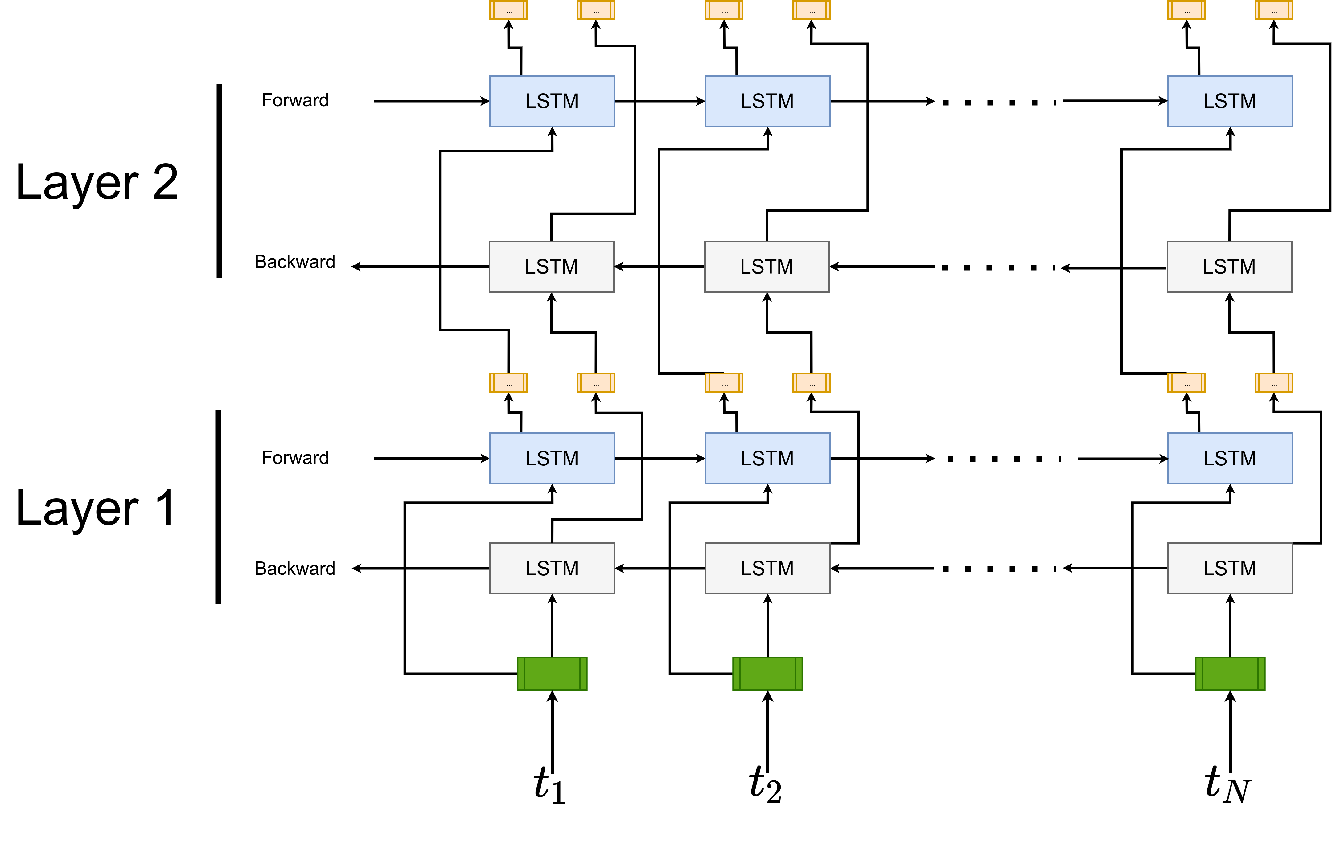

ELMo is a task specific combination of the intermediate layer representations in the biLM. Higher-level LSTM states capture context-dependent aspects of word meaning (word sense disambiguation tasks) while lower level states model aspects of syntax (POS tagging). For each token \(t_k\), a L-layer biLM computes a set of \(2L+1\) representations (forward + backward + \(x_k\))

\[R_k = \{\mathbf{x}_{k}^{LM}, \vec{\mathbf{h}}_{k,j}^{LM}, \overleftarrow{\mathbf{h}}_{k,j}^{LM} \mid j=1, 2, ..., L\}\] \[= \{\mathbf{h}_{k,j}^{LM} \mid j=0, 1, ..., L\}\]

where \(\mathbf{h}_{k,0}^{LM}\) is the token layer and \(\mathbf{h}_{k,j}^{LM} = [\vec{\mathbf{h}}_{k,j}^{LM};\overleftarrow{\mathbf{h}}_{k,j}^{LM}]\), for each biLSTM layer. For inclusion in a downstream model, ELMo collapses all layers in \(R\) into single vector, \(\mathbf{\text{ELMo}_k} = E(R_k; \Theta_e)\). In the simplest case, ELMo just selects the top layer \(E(R_k) =\mathbf{h}_{k,l}^{LM}\).

BERT

References

[1] Speech and Language Processing (2nd Edition), Jurafsky, Daniel and Martin, James H. 2009. Prentice-Hall, Inc. ISBN: 0131873210

[2] Linguistics: An Introduction to Linguistic Theory Victoria, A. Fromkin, 2011. ISBN: 0631197117

[3] Distributed Representations of Words and Phrases and their Compositionality, Mikolov et al., 2013. arXiv: 1310.4546

[4] Efficient Estimation of Word Representations in Vector Space, Mikolov et al., 2013. arXiv: 1301.3781

[5] Learning word embedding. Weng, Lilian, 2017. URL: https://lilianweng.github.io/lil-log/2017/10/15/learning-word-embedding.html

[6] GloVe: Global Vectors for Word Representation, Pennington et al., 2014

[7] Enriching Word Vectors with Subword Information, Bojanowski et al., 2016. arXiv: 1607.04606

[8] Natural Language Processing with Deep Learning CS224N/Ling284, Christopher Manning, Lecture 2. URL: http://web.stanford.edu/class/cs224n/slides/cs224n-2021-lecture02-wordvecs2.pdf

[9] Linear Algebraic Structure of Word Senses, with Applications to Polysemy, Arora et al., 2016. arXiv: 1601.03764

[10] Deep contextualized word representations, Peters et al., 2018. arXiv: 1802.05365