Dune Embeddings
Consider this as an unorthodox way to recommend Dune.
This blog post covers some experimental word embeddings on the book series called Dune. I am writing this post just for fun. As you may know that, Dune has distinctive linguistic features (the universal language in Dune Universe is Galach), mostly based on varieties of Arabic. I trained a corpus of six main books of Dune: Dune (1), Dune Messiah (2), Children Of Dune (3), God Emperor Of Dune (4), Heretics of Dune (5), Chapterhouse Dune (6).
As you may know, word2vec [1] is proposed in the paper called Distributed Representations of Words and Phrases and their Compositionality (Mikolov et al., 2013). It allows you to learn the high-quality distributed vector representations that capture a large number of precise syntactic and semantic word relationships. Word2vec algorithm uses Skip-gram Mikolov et al., 2013 model to learn efficient vector representations. Those learned word vectors has interesting property, words with semantic and syntactic affinities give the necessary result in mathematical similarity operations. In Skip-gram connections we have an objective to minimize:
\[\max \limits_{\theta} \prod_{\text{center}} \prod_{\text{context}} p(\text{context}|\text{center} ;\theta)\] \[= \max \limits_{\theta} \prod_{t=1}^T \prod_{-c \leq j \leq c, j \neq c} p(w_{t+j}|w_t; \theta)\] \[= \min \limits_{\theta} -\frac{1}{T} \prod_{t=1}^T \prod_{-c \leq j \leq c, j \neq c} p(w_{t+j}|w_t; \theta)\] \[= \min \limits_{\theta} -\frac{1}{T} \sum_{t=1}^T \sum_{-c \leq j \leq c, j \neq c} \log p(w_{t+j}|w_t; \theta)\]The term center and context can be expressed as an example (with a fixed window size): w = “to learn word vector representations”
| x (center) | y (context) |
|---|---|
| word (w2) | learn (w1) |
| word (w2) | vector (w3) |
| vector (w3) | word (w2) |
| vector (w3) | representations (w4) |
Skip-gram objective is to find word representations that are useful for predicting the surrounding words in a sentence or a document. We maximize the probability of “this words (context) for these word (center)”. Of course, increased fixed window size can give us better accuracy.
How can we calculate those probabilities? With a single softmax?
\[p(w_O, | w_I) = \frac{\exp(V_{w_O}' V_{w_I}^T)}{\sum_{w'=1}^{\mid V \mid} \exp(V_{w'} V_{w_I}^T)}\]This softmax is class probability of context words in the entire vocabulary, we maximize this class probabilities. But this is impractical due to the cost of computing gradient of this term is proportional to size of our vocabulary V, which is about 60k in our case. In order to computational efficiency, we use a simplified version of Noise Constrastive Estimation: Negative Sampling. This Negative Sampling objective is defined as
\[\log \sigma(V_{w_O}' V_{w_I}^T) + \sum_{i=0}^{k} \mathbb{E}_{w_i \sim P_n(w)} \left[\log \sigma(- V_{w_i}' V_{w_I}^T) \right]\]This objective says that, “I want to classify the word sampling against the other classes higher”. The term \(V_{w_O}'\) is for “word around it”, the term \(V_{w_I}\) is for “word I considered”. The sampling \(w_i \sim P_n(w)\) means “sample word from your vocabulary at random and sample \(k\) of them”. When you maximize this objective, you also minimize the summation term. But what is \(P(w_i)\)?
Authors of the paper said that, in very large corpora, the most frequent words can easily occur hundreds of millions of times. Such words usually provide less information value than the rare words. For example, while the Skip-gram model benefits from observing co-occurrences of “Fremen” and “Crysknife”, it benefits much less from observing the frequent co-occurrences of “Fringe” and “the”, as nearly every word co-occurs frequently within a sentence “the”. To counter the imbalance between the rare and frequent words, such a subsampling approach is proposed:
\[P(w_i) = 1 - \sqrt{\frac{t}{frequency(w_i)}}\]Where \(t\) is the temperature, chosen \(10^{-5}\). This formulation aggressively subsamples words whose frequency is greater than t while preserving the ranking of the frequencies.
Let’s play with Dune Embeddings. Firstly, as always, you cannot escape from it, we have imports:
from gensim.models import Word2Vec
from time import time
import re
import pandas as pd
import numpy as np
from collections import defaultdict
import spacy
import nltk
from gensim.models.phrases import Phrases, Phraser
from nltk.tokenize import word_tokenize
from nltk.tokenize import sent_tokenize
nltk.download('punkt')
import warnings
Then we read our book data, served as .txt file. We apply nltk’s sentence tokenizer sent_tokenize() to tokenize the sentences in this text files.
with open(base+'dune2.txt') as f1:
  data1 = f1.read()

with open(base+'dune3.txt') as f2:
  data2 = f2.read()

with open(base+'dune4.txt') as f3:
  data3 = f3.read()

with open(base+'dune5.txt') as f4:
  data4 = f4.read()

with open(base+'dune6.txt') as f5:
  data5 = f5.read()

with open(base+'dune7.txt') as f6:
  data6 = f6.read()

data1 = sent_tokenize(data1)
data1 = pd.DataFrame(data1,columns=['sentences'])
data2 = sent_tokenize(data2)
data2 = pd.DataFrame(data2,columns=['sentences'])
data3 = sent_tokenize(data3)
data3 = pd.DataFrame(data3,columns=['sentences'])
data4 = sent_tokenize(data4)
data4 = pd.DataFrame(data4,columns=['sentences'])
data5 = sent_tokenize(data5)
data5 = pd.DataFrame(data5,columns=['sentences'])
data6 = sent_tokenize(data6)
data6 = pd.DataFrame(data6,columns=['sentences'])

frames = [data1, data2, data3, data4, data5, data6]
data = pd.concat(frames)
From now, we use spacy for other processing techniques. When you call nlp on a text, spacy first tokenizes the text to produce a Doc object. The Doc is then processed in several different steps. This is also referred to as the processing pipeline. We’ll disable all other statistical components (in this case, parser) during processing for speed. Then we lemmatize the words and remove stop words.
nlp = spacy.load('en', disable=['parser'])

def preprocess(doc):
    txt = [token.lemma_ for token in doc if not token.is_stop] # doc \in spacy.doc object
    if len(txt) > 2:
        return ' '.join(txt)

data_preprocess = (re.sub("[^A-Za-z']+", ' ', str(row)).lower() for row in data['sentences']) # removes non-alphabetic characters
txt = [preprocess(doc) for doc in nlp.pipe(data_preprocess, batch_size=5000, n_threads=-1)]
df_cleaned = pd.DataFrame({'cleaned': txt})
df_cleaned = df_cleaned.dropna().drop_duplicates()
In function preprocess(), we also not to choose sentences longer than 2. Word2Vec uses context words to learn the vector representation of a target word, if a sentence is only one or two words long, the benefit for the training is very small. We use regular expression to remove non-alphabetic characters for each line.
Other processing technique is detect common phrases (bigrams). For example Muad Dib is a bigram that is very useful for Dune context. Or bigram Bene Gesserit is indispensable. We use gensim to automatically detect common phrases (bigrams) from a list of sentences.
sentence = [row.split() for row in df_cleaned['cleaned']]
phrases = Phrases(sentence, min_count=30, progress_per=10000)
sentences = phrases[sentence];
Then we calculate the frequencies.
word_freq = defaultdict(int)
for sent in sentences:
    for i in sent:
        word_freq[i] += 1
Now it is time to create our word2vec model. We set up the parameters of the model one-by-one.
word2vec = Word2Vec(min_count=20,
                     window=2,
                     size=300,
                     sample=6e-5,
                     alpha=0.03,
                     min_alpha=0.0007,
                     negative=20,
                     workers=cores-1)
Hyperparameters that we learned:
- min_count: Ignores all words with total absolute frequency lower than this.
- window: The maximum distance between the current and predicted word within a sentence. (as you can see in the paper)
- size: Dimensionality of the feature vectors.
- sample: The threshold for configuring which higher-frequency words are randomly downsampled. (as you can see in the paper)
- alpha: The initial learning rate
- in_alpha: changing learning rage
- negative: negative sampling, the int for negative specifies how many “noise words” should be drown.
Then, we initialized our model with building the vocabulary from a sequence of sentences.
word2vec.build_vocab(sentences, progress_per=10000)
Finally let’s train our word2vec model.
word2vec.train(sentences, total_examples=w2v_model.corpus_count, epochs=30, report_delay=1)
w2v_model.init_sims(replace=True)
Let’s play!

FIGURE: Reverend Mother Gaius Mohiam (a Bene Gesserit) while testing Paul Atreides with a Gom Jabbar.
What are the most similiar 10 word of bene gesserit? (explanation: The Bene Gesserit are a powerful and ancient order of women that are trained as a most patient, high analytical and more).
word2vec.wv.most_similar(positive=["bene_gesserit"])
Output:
[('superior', 0.9340497255325317),
 ('teaching', 0.9308292865753174),
 ('teacher', 0.9248643517494202),
 ('sisterhood', 0.9196563959121704),
 ('bene_tleilax', 0.9170730113983154),
 ('analysis', 0.9170225858688354),
 ('education', 0.9143076539039612),
 ('breeding_program', 0.9017256498336792),
 ('alliance', 0.90071702003479),
 ('fact', 0.8998515009880066)]

FIGURE: A Fremen.
What are the most similiar 10 word of fremen? (explanation: Fremens are native race of the planet Dune. Muad’Dib’s Jihad launched by Paul Atreides, their adopted leader and more)
word2vec.wv.most_similar(positive=["fremen"])
Output:
[('spirit', 0.9168293476104736),
 ('paradise', 0.9119386672973633),
 ('legend', 0.9027668833732605),
 ("muad'dib", 0.9022884368896484),
 ('prophet', 0.8965635895729065),
 ('demon', 0.8792929649353027),
 ('soul', 0.8790735602378845),
 ('world', 0.8738502264022827),
 ('commentary', 0.8680400848388672),
 ('folk', 0.8670632243156433)]
What are the most similiar 10 word of lisan? (explanation: Lisan al Gaib is the Fremen term for an off-world prophet. and more)
word2vec.wv.most_similar(positive=["lisan"])
Output:
[('gaib', 0.9857056140899658),
 ('harq', 0.9847873449325562),
 ('al', 0.9727405309677124),
 ('ada', 0.9507930874824524),
 ('legend', 0.9193408489227295),
 ('world', 0.8181276321411133),
 ('flee', 0.7918423414230347),
 ('atreides', 0.789204478263855),
 ('commentary', 0.7849634885787964),
 ("muad'dib", 0.7831201553344727)]
What are the most similiar 10 word of spice? (explanation: The Spice Melange, commonly referred to simply as ‘the spice’, was a naturally produced awareness spectrum narcotic that formed a fundamental block of commerce and technological development in the known universe for millennia and more)
word2vec.wv.most_similar(positive=["spice"])
Output:
[('melange', 0.9448734521865845),
 ('essence', 0.8954010009765625),
 ('rich', 0.8934587240219116),
 ('mass', 0.881293773651123),
 ('pre', 0.8805406093597412),
 ('diet', 0.8717115521430969),
 ('food', 0.8487979173660278),
 ('addiction', 0.8199436068534851),
 ('trace', 0.8126449584960938),
 ('growth', 0.8088463544845581)]
What are the most similiar 4 word of choam? (explanation: essentially controls all economic affairs across the cosmos and more)
word2vec.wv.most_similar(positive=["choam"])
Output:
[('great_house', 0.9707689881324768),
 ('landsraad', 0.9658929109573364),
 ('profit', 0.9448226690292358),
 ('company', 0.9420391321182251)]
What are the most similiar 4 word of qanat? (explanation: Open canal for carrying irrigation water under controlled conditions through a desert)
word2vec.wv.most_similar(positive=["qanat"])
Output:
[('pole', 0.9524651765823364),
 ('planting', 0.9271722435951233),
 ('river', 0.9262102246284485)]

FIGURE: Flag of House Atreides.
And, lastly, for the glory of House Atreides, what are the most similiar 10 word of atreides? (explanation: House Atreides was one of the Houses Major within the infrastructure of the Galactic Padishah Empire. They were ruled by the patriarch of the Atreides family, who took the title of Duke and more)
word2vec.wv.most_similar(positive=["atreides"])
Output:
[('father', 0.9062684178352356),
 ('son', 0.8857165575027466),
 ('custom', 0.8835201263427734),
 ('cousin', 0.8806978464126587),
 ('atreide', 0.8775589466094971),
 ('planetologist', 0.8765182495117188),
 ("muad'dib", 0.8737363815307617),
 ('grandfather', 0.8719019889831543),
 ('title', 0.8706281185150146),
 ('family', 0.8610590696334839)]
t-SNE
t-SNE (Maaten et al., 2008) is a non-linear dimensionality reduction algorithm that attempts to represent high-dimensional data and the underlying relationships between vectors in a lower-dimensional space.
Let’s plot our vectors.
import numpy as np
import matplotlib.pyplot as plt
%matplotlib inline
import seaborn as sns
sns.set_style("darkgrid")
from sklearn.decomposition import PCA
from sklearn.manifold import TSNE

def tsnescatterplot(model, word, list_names):
    arrays = np.empty((0, 300), dtype='f')
    word_labels = [word]
    color_list  = ['red']
    arrays = np.append(arrays, model.wv.__getitem__([word]), axis=0)# adds the vector of the query word
    close_words = model.wv.most_similar([word])# gets list of most similar words

    for wrd_score in close_words:
        wrd_vector = model.wv.__getitem__([wrd_score[0]])
        word_labels.append(wrd_score[0])
        color_list.append('blue')
        arrays = np.append(arrays, wrd_vector, axis=0)

    for wrd in list_names:
        wrd_vector = model.wv.__getitem__([wrd])
        word_labels.append(wrd)
        color_list.append('green')
        arrays = np.append(arrays, wrd_vector, axis=0)

    reduc = PCA(n_components=19).fit_transform(arrays) # Reduces the dimensionality from 300 to 19 dimensions with PCA
    np.set_printoptions(suppress=True)# Finds t-SNE coordinates for 2 dimensions
    Y = TSNE(n_components=2, random_state=0, perplexity=15).fit_transform(reduc)

    df = pd.DataFrame({'x': [x for x in Y[:, 0]],
                       'y': [y for y in Y[:, 1]],
                       'words': word_labels,
                       'color': color_list})
    fig, _ = plt.subplots()
    fig.set_size_inches(9, 9)
    p1 = sns.regplot(data=df,
                     x="x",
                     y="y",
                     fit_reg=False,
                     marker="o",
                     scatter_kws={'s': 40,
                                  'facecolors': df['color']
                                 }
                    )
    for line in range(0, df.shape[0]):
         p1.text(df["x"][line],
                 df['y'][line],
                 '  ' + df["words"][line].title(),
                 horizontalalignment='left',
                 verticalalignment='bottom', size='medium',
                 color=df['color'][line],
                 weight='normal'
                ).set_size(15)

    plt.xlim(Y[:, 0].min()-50, Y[:, 0].max()+50)
    plt.ylim(Y[:, 1].min()-50, Y[:, 1].max()+50)
    plt.title('t-SNE visualization for {}'.format(word.title()))
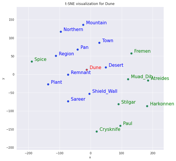
10 most similar words versus 8 random words for word Dune
tsnescatterplot(word2vec, 'dune', ['fremen', 'atreides',
'harkonnen', 'paul', 'crysknife', 'spice', 'muad_dib', 'stilgar'])
Output:

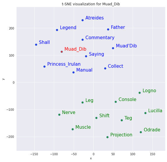
10 most similar words versus 10 most dissimilar for word muad_dib
tsnescatterplot(w2v_model, 'muad_dib',
[i[0] for i in w2v_model.wv.most_similar(negative=["muad_dib"])])
Output:

Conclusion
“I must not fear. Fear is the mind-killer. Fear is the little-death that brings total obliteration. I will face my fear. I will permit it to pass over me and through me. And when it has gone past I will turn the inner eye to see its path. Where the fear has gone there will be nothing. Only I will remain.”
Read Dune.
References
- Distributed Representations of Words and Phrases and their Compositionality (Mikolov et al., 2013)
- Efficient Estimation of Word Representations in Vector Space (Mikolov et al., 2013)
- Pytorch Implementation of Word2Vec
- Language Processing Pipelines
- models.word2vec – Word2vec embeddings
- Visualizing Data using t-SNE (Maaten et al., 2008)
- Inzva’s Applied AI Word2Vec Section


Leave a comment