A Survey On Music Generation With Deep Neural Networks

Abstract

Music is an art of time. It is formed by the colaboration of instruments -composed with many instruments collectively- harmonization of notes. So, music generation with deep neural networks strictly connected with this features of music. There are many models have been proposed so far for generating music. Some of them based on the structure of Recurrent Neural Networks or Generative Adversarial Networks or Variational Autoencoders. We will see that different models use different representation of music like piano-roll representation, different representation of it’s temporal structure for synthetic music. In this post, we will examine those models detailed.

Generating Music With Recurrent Neural Networks

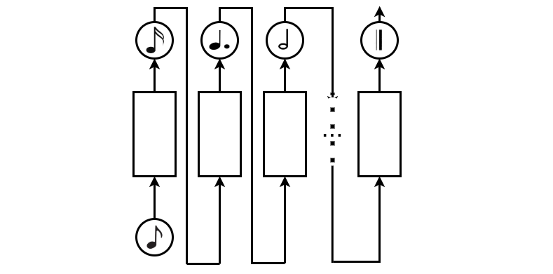
Recurrent Neural Networks are very simple way to represent sequential data like music. RNNs learns a probability distribution over the next notes given all the previous notes. We have to give an training data to the model, which can be either audo file or symbolic representation of music. MIDI itself does not make sound, it is just a series of messages like “note on,” “note off,” “note/pitch,” “pitch-bend,” and many more. These messages are interpreted by a MIDI instrument to produce sound. A software called Music21 can transform midi file into textual chord form (A,B,C etc.). One can easily get the notes from mid file and convert it to sequential data to use with RNNs:

From this script

from midihelper import getNotes, noteToSequence
def main():
    notes = getNotes('/path/to/midi.mid')
    seqdata = noteToSequence(notes,len(set(notes)))

if __name__ == '__main__':
    main()

Generating Music With Generative Adversarial Networks

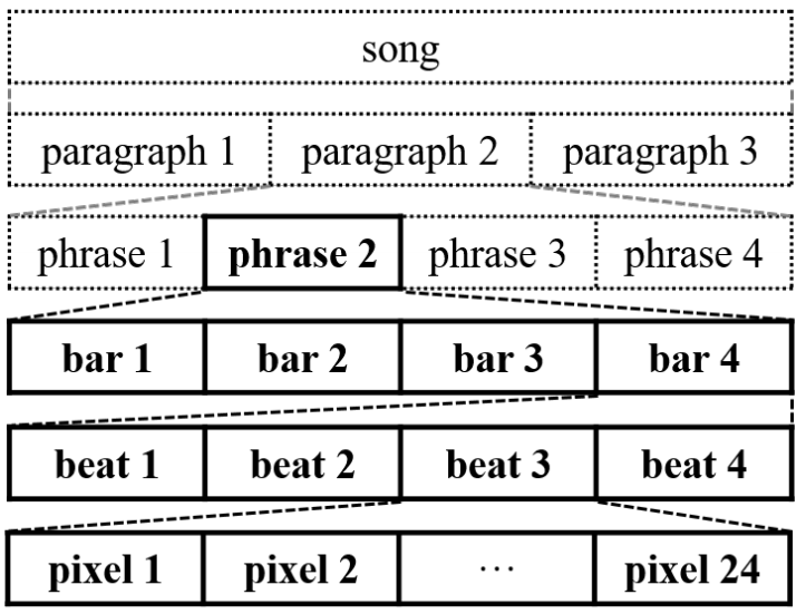
MuseGAN is a Generative Adversarial Network for music generation. It uses piano-roll representation of MIDI files. A piano-roll dataset called Lakh is used for MuseGAN. But what is piano-roll? The Lakh Pianoroll Dataset (LPD) is a collection of 174,154 multitrack pianorolls derived from the Lakh MIDI Dataset (LMD). The dataset contains 5 dimensions. (30,887 X number of bars X time step by a bar (96) X notes in roll [pitches] (128) X tracks (instruments)). The term bar has same meaning with bar in music.

Bar In Lakh	Bar In Music

MuseGAN has 3+2 proposals. The first three represent different techniques to generate tracks (instruments). The last two represent different techniques to represent temporal structure of music.

Jamming Model

Figure source [3]

Multiple generators work independently and generate music of its own instrument. The generators receive critics from different discriminators. It can be seen as, different instrument players improvize in different studios. Like free jazz (!). They can’t hear each other but they create a song collectively.

Composer Model

Figure source [3]

One single generator creates multi-channel pianoroll with each channel representing a specific instrument. This model requires only one shared random vector (like conducting) and one discriminator.

Hybrid Model

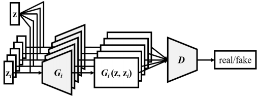
Figure source [3]

Combining the idea of jamming and composer models. Generator takes input as inter-track \(z\) and a intra-track \(z_i\). Inter-track can coordinate the generation of different instruments like composer does. And one discriminator to evaluate instruments collectively. It can be seen as; every instrument has its own individuality, at the sime time, each instrument creates a song collectively by hearing each other.

Track Unconditional Temporal Model

Figure source [3]

Generating bars with coherence among the bars. Temporal structure generator \(G_{\text{temp}}\), bar generator \(G_{\text{bar}}\). \(G_{\text{temp}}\) maps noise vector \(z\) to sequence of latent vectors. \(G_{\text{bar}}\) is used for generating pianorolls sequentially.

\[G(z) = \{G_{\text{bar}}(G_{\text{temp}}(z)^{(t)})\}_{t=1}^T\]

Track Conditional Temporal Model

Figure source [3]

The vector y is given by human and tries to learn the temporal structure underlying that instrument and to generate the remaining tracks. One can add a encoder to achieve such conditional generation with highdimensional conditions, an additional encoder \(E\) is trained.

\[G^{\circ}(z,y) = \{G^{\circ}_{\text{bar}}(z^{(t)}, E(y^{(t)}))\}_{t=1}^T\]

The Model

Figure source [3]

MuseGAN is an integration and extension of the proposed models that we discussed. Input is composed into 4 parts. Inter-track time-independent random vectors \(z\), intra-track time-independent vectors \(z_i\), inter-track time-dependent random vectors \(z_t\), intra-track time-dependent random vectors \(z_{i, t}\). Index \(i\) is for instruments, index \(t\) is for sequence of time.

\[G(\hat{z}) = \{ G_{\text{bar},i} (z, G_{\text{temp}}(z_t)^{(t)}, z_i, G_{\text{temp},i}(z_{i,t})^{(t)})\}_{i,t=1}^{M,T}\]

Jukebox

JukeBox is a generative model for music with singing that is based on Vector Quantized Variational Autoencoders. The models use raw audio (.wav) for training data. We implemented an upsampling section and created music based on different styles.

Earlier models have been applied to music generation tasks. As we discussed they generated music symbolically in the form of a piano roll; which specifies the timing, velocity, pitch and notes of each instrument. Or in the form of a MIDI file to textual representation. The symbolic way has lower dimensional space than raw audio. However, the symbolic way constrains the music. A way to reduce the curse of dimensionality is learn a lower-dimensional encoding of raw audio.

Vector Quantized Variational Autoencoders

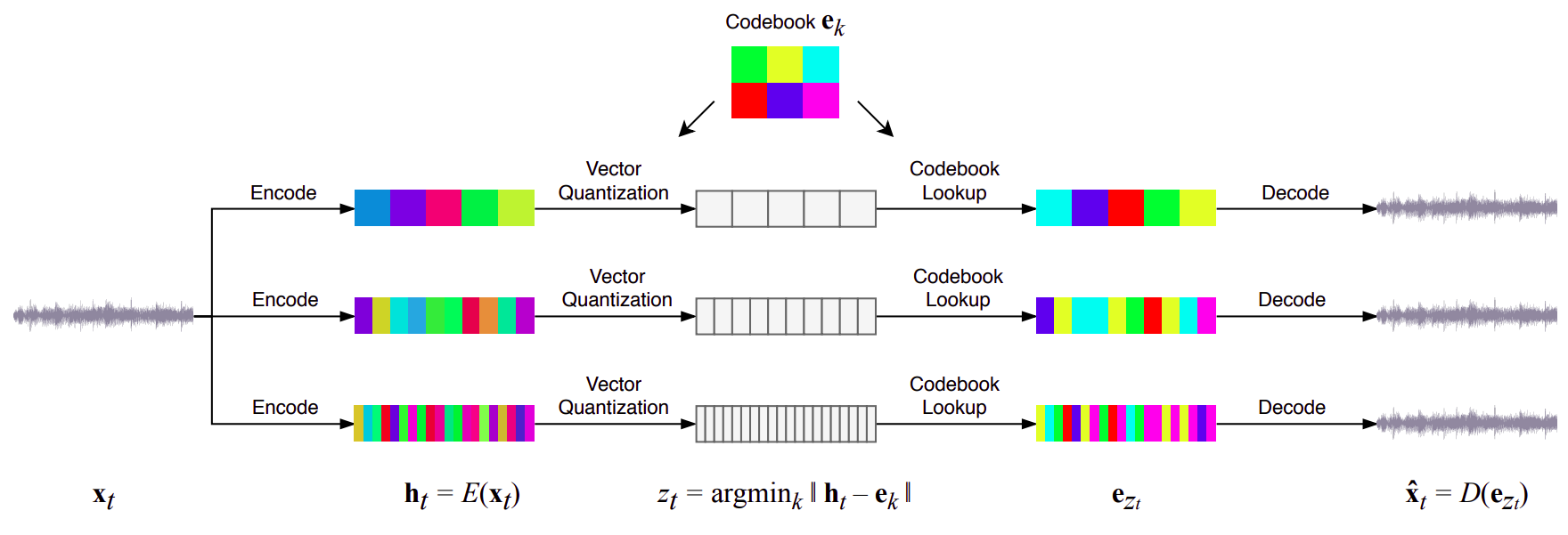
Figure source [1]

Jukebox is a combination of Vector Quantized Variational Autoencoder (VQ-VAE) and Transformers, that is trained on 1.2 million songs (32 bits of information, 44.1 kHz. sampling rate, randomly downmixing the right and left channels) with paired lyrics and metadata from LyricWiki.

Raw audio is represented as a continuous waveform x ∈ [-1, 1]T where the number of samples T is the product of the audio duration t and the sampling rate, typically 16 kHz to 48 kHz. Input of the Vector Quantized Variational Autoencoder is this continuous waveform derived from provided raw audio.

Upsampling Strategies

Ancestral Sampling	Windowed \& Primed Sampling

Figure source [1]

Similar to other well-known applications of VQ-VAE’s, to optimize knowledge distillation, Jukebox exploits use of varying hop lengths for seperate VAE’s. Yet, even this strategy provides different levels of understanding of raw audio, harmonizing results from separate encoders to achieve a common task is quite challenging and somehow experimental. Jukebox employs three different sampling approaches to harvest and transfer each level’s knowledge: ancestral, windowed and primed sampling. Use of these methods is up to the aim of the given task such as windowed sampling is a must for longer music generation whereas primed sampling is quite advantageous when a piece of track is provided beforehand.

Prior Model

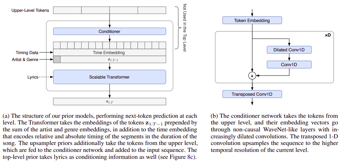
Figure source [1]

At the heart of the Jukebox, the prior model is responsible for collecting samples from upper levels, conditioning them to external factors (e.g. timing, artist, genre and lyrics) and performing next-token prediction task thanks to the built-in scalable transformer. The conditioning operation is performed by a conditioner network consisting of many WaveNet-like convolutions with increasing dilation. Moreover, the scope of the external factors up to the sensitivity of the model, and since they are just naive transformer embeddings, the extent of the upsampling could freely be set.

Scalable (Sparse) Transformer

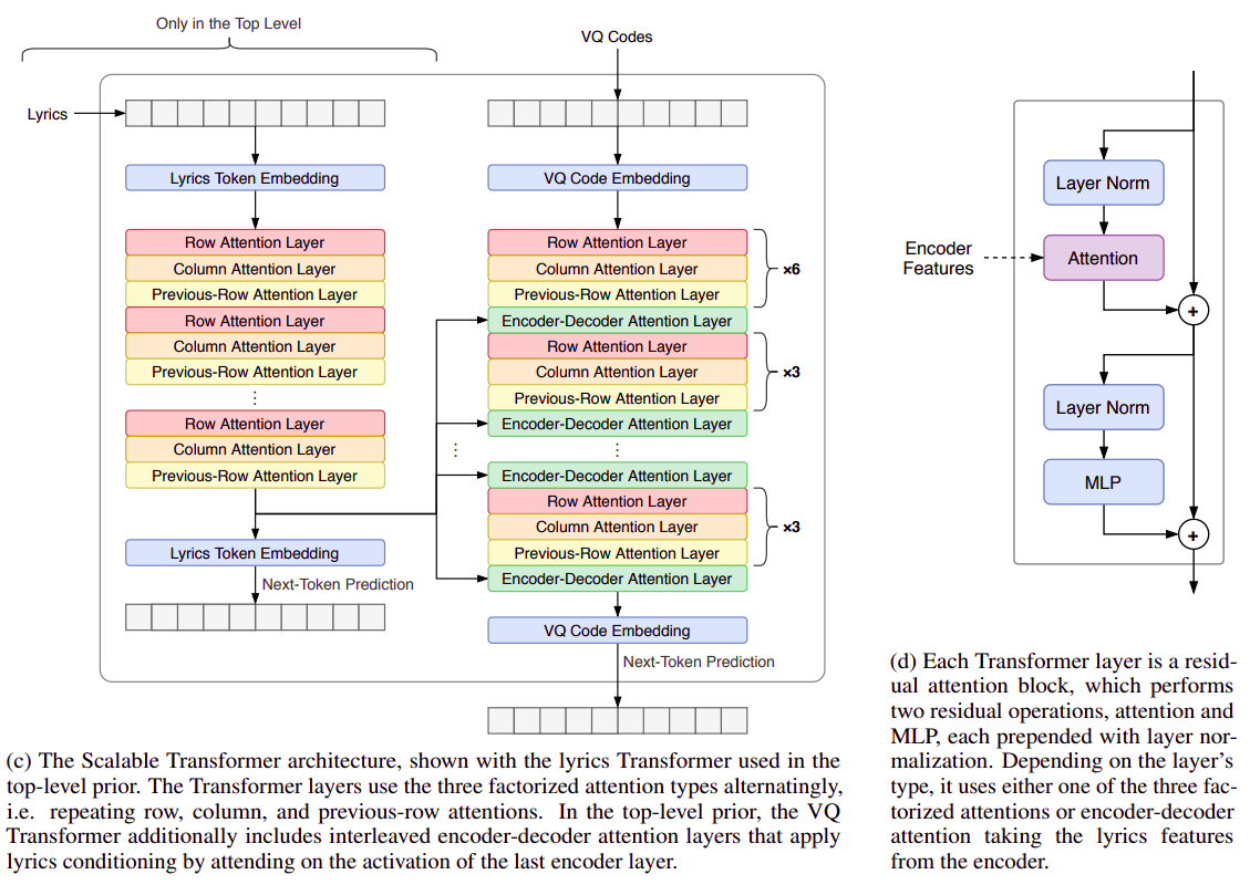
Figure source [1]

Most of the operation is performed by the Scalable Transformer within the prior model, which forms the performance bottleneck of the model. In addition to the common transformer architectures, Jukebox utilizes specific attention mechanisms (e.g. row, column and previous-row attentions) in residual layers to achieve perfect context-music harmony, which costs far more than the naive transformers. Other than the use of various attention strategies, residual layers are analogous to any other transformer architecture, in other words, the original structure is preserved.

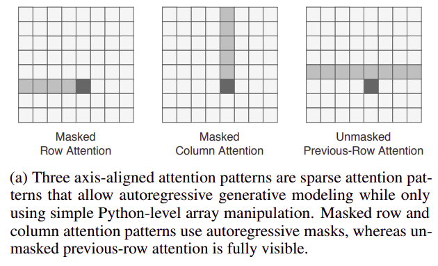
Figure source [1]

Results

Training is performed on the prior model, which is conditioned on the external factors provided accordingly, and exploited the audio-features of the raw audio files by use of separate VQ-VAE’s with varying hop lengths. The load of the training is tremendous in parallel with the expectations from the model, yet, results are promising in contrast with the novelty of the extent of the work. Despite the absence of robust metrics due to lack of prior work, provided examples show that being optimistic in results is fair.

Please see the success of the Jukebox in terms of genre/style conditioning:

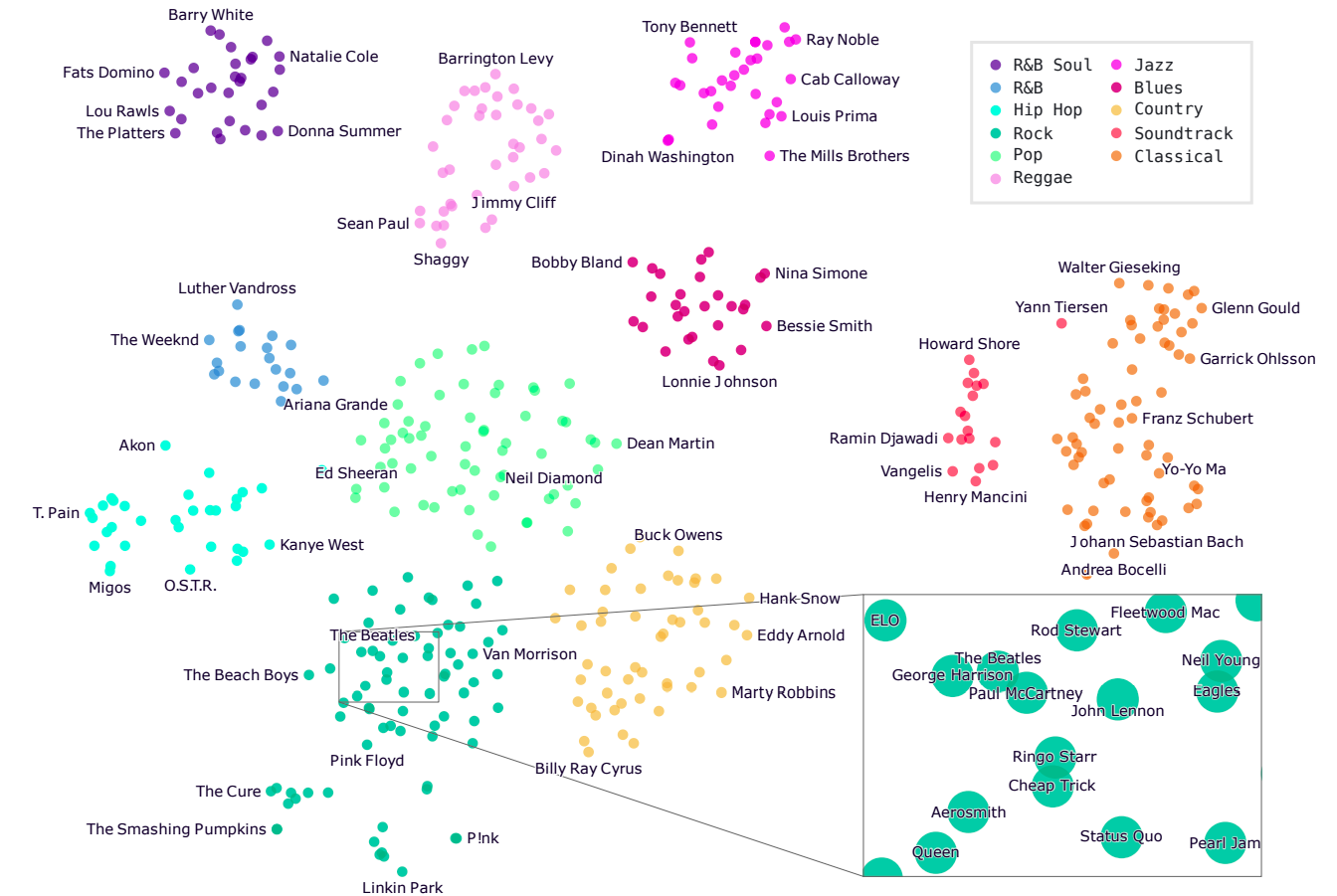
Figure source [1]

Generated Samples

• Artist: Steven Wilson, Genre: Synthwave

• Artist: Nirvana, Genre: Acoustic, Lyrics: Alice In Chains - Love, Hate, Love

• Artist: Alice In Chains, Genre: Acoustic
• Lyrics:

Train what you want to overfit

See that big graphics card

We love inzva, we love inzva

I don’t like cuda memory error

References

[1] Prafulla Dhariwal, Heewoo Jun, Christine Payne, Jong Wook Kim, Alec Radford, Ilya Sutskever. Jukebox: A Generative Model for Music. URL: https://cdn.openai.com/papers/jukebox.pdf

[2] Aaron van den Oord, Oriol Vinyals, Koray Kavukcuoglu. Neural Discrete Representation Learning. URL: https://arxiv.org/pdf/1711.00937.pdf

[3] Hao-Wen Dong, Wen-Yi Hsiao, Li-Chia Yang, Yi-Hsuan Yang. MuseGAN: Multi-track Sequential Generative Adversarial Networks for Symbolic Music Generation and Accompaniment. URL: https://arxiv.org/pdf/1709.06298.pdf

[4] Gullapalli Keerti, A N Vaishnavi, Prerana Mukherjee, A Sree Vidya, Gattineni Sai Sreenithya, Deeksha Nayab. Attentional networks for music generation. URL: https://arxiv.org/pdf/2002.03854.pdf

[5] Nikhil Kotecha, Paul Young. Generating Music using an LSTM Network. URL: https://arxiv.org/pdf/1804.07300.pdf

Project Collaborators

• Şafak Bilici
• Yüşa Ömer Altıntop
• Onur Boyar